Evaluating the Arrhenius equation for developmental processes

Abstract

The famous Arrhenius equation is well suited to describing the temperature dependence of chemical reactions but has also been used for complicated biological processes. Here, we evaluate how well the simple Arrhenius equation predicts complex multi-step biological processes, using frog and fruit fly embryogenesis as two canonical models. We find that the Arrhenius equation provides a good approximation for the temperature dependence of embryogenesis, even though individual developmental intervals scale differently with temperature. At low and high temperatures, however, we observed significant departures from idealized Arrhenius Law behavior. When we model multi-step reactions of idealized chemical networks, we are unable to generate comparable deviations from linearity. In contrast, we find the two enzymes GAPDH and β-galactosidase show non-linearity in the Arrhenius plot similar to our observations of embryonic development. Thus, we find that complex embryonic development can be well approximated by the simple Arrhenius equation regardless of non-uniform developmental scaling and propose that the observed departure from this law likely results more from non-idealized individual steps rather than from the complexity of the system.

Keywords: Drosophila melanogaster; Xenopus laevis; Arrhenius equation; embryonic development; temperature dependence.

Figure 1. Temperature dependence of development progression in fly and frog embryos

1. A table representing D. melanogaster developmental scoring event names and sequential score codes used throughout this paper.

2. X. laevis developmental scoring and codes used throughout this paper.

3. Shown here is a schematic depicting how time $\left(\tau \right)$ intervals are determined based on beginning and ending scores. Plotted also are all mean time intervals from t = 0, defined as 14^th syncytial cleavage, to reach various developmental scores in D. melanogaster embryos. Error bars in time indicate standard deviation among replicates (n = 2–13 biological replicates per temperature). Error bars in temperature represent the standard error (± 0.5°C) of the thermometer used when recording temperature.

4. As (C) but for X. laevis, since t = 0 (3^rd cleavage) at temperatures ranging from 10.3°C to 33.1°C (n = 1–23 biological replicates per temperature).

Figure EV1. Scored developmental events and coefficient of variation (CV) analysis

1. Sketches of 12 developmental scores determined to be the most reproducible, in D. melanogaster. Please see Materials and Methods and Movie EV1 for definition of scoring criteria.

2. Seven additional developmental events in fly embryos that we did not pursue due to poor reproducibility i.e. cut score. The number score code is used in the following CV analysis.

3. We calculated CVs using preliminary data for every developmental time interval between the 19 scores (described in Materials and Methods) we considered investigating (Dataset EV1). CVs are calculated for each of the 6 different temperatures (n = 3–5 biological replicates per temperature), and the mean CV is then displayed for each interval. CV’s are displayed as percentages. The 11 most reproducible intervals for neighboring scores (diagonal) are shown in green. Intervals shown in red had their associated score (numbers) cut from our investigation.

4. Sketches of 12 developmental event we investigated in X. laevis determined most reproducible. Please see Materials and Methods and Movie EV2 for definition of scoring criteria.

5. As (B) but for four additional frog developmental events not included in our final analysis.

6. As (C) but for intervals calculated from early data, between 16 frog developmental scores considered (described in Material and Methods) averaged over 16 temperatures (n = 2–6 biological replicates per temperature) (Dataset EV2). The 11 most reproducible intervals for neighboring scores (diagonal) are shown in green.

Figure 2. Apparent activation energies vary significantly between developmental intervals

1. Arrhenius plots for two examples of developmental intervals (D–E, E–F) in D. melanogaster. Blue data points are the means of replicates for viable temperatures that survive until First Breath. Red data represent more extreme temperature values where embryos do not survive until First Breath. A linear regression (solid black line, n = 66, 65 independent biological measurements, respectively) was fit over the core temperature range (14.3–27°C), from which E_a was calculated and reported with its 68% confidence interval. Error bars in temperature represent the standard error (± 0.5°C) of the thermometer used when recording temperature. Error bars in ln(rate) represent standard error (n = 3–13 biological replicates).

2. As (A) but for intervals G‐H, K‐L in X. laevis. Blue data points represent viable temperatures where embryos survive until Late Neurulation. A linear regression (solid black line, n = 120, 94 independent biological measurements, respectively) was fit over core temperatures spanning 12.2–25.7°C, from which the E_a was calculated and reported in black. Error bars in temperature represent the standard error (± 0.5°C) of the thermometer used when recording temperature. Error bars in ln(rate) represent standard error (n = 1–10 biological replicates).

3. Apparent activation energies in fly calculated from Arrhenius plots (Fig EV2A). The x‐axis is labeled with the developmental interval, marked by start and endpoint. Error bars represent the 68% confidence interval for the activation energy based on linear fit in the Arrhenius plot. Black braces connect examples of developmental intervals that show statistically significant differences in slope (and thus E_a), with respectable power (> 0.8), ***P < 0.001, (F‐test), (n = 39–60 independent biological measurements).

4. As (C) but for frog E_a calculated from plots shown in Fig EV2B. Magenta brackets represent groupings (all points above the bracket) showing no statistical difference (#) in activation energy (F‐test), (n = 94–135 independent biological measurements).

Figure EV2. Arrhenius plots for fly and frog

1. Shown are Arrhenius plots (similar to Fig 2A) for developmental intervals between 12 adjacent fly developmental scores. Linear fits (solid black line) were calculated from 14.3 to 27°C. The apparent activation energy for each interval is displayed top right of each subplot. Blue data points represent temperatures viable until First Breath. Extreme temperatures that do not survive until our final scores are shown in red. A quadratic (dashed red line) is fit through all the data (red and blue). Error bars in temperature represent the standard error (± 0.5°C) of the thermometer used when recording temperature. Error bars in ln(rate) represent standard error (n = 2–13 biological replicates per temperature).

2. As (A) but using 12 adjacent frog developmental scores. Linear fits are calculated from 12.2 to 25.7°C, used in Fig 2B, (n = 1–23 biological replicates per temperature). Blue data points represent temperatures viable until Late Neurulation.

Figure EV3. Reanalysis of temperature dependence data in Drosophila melanogaster development from Kuntz and Eisen

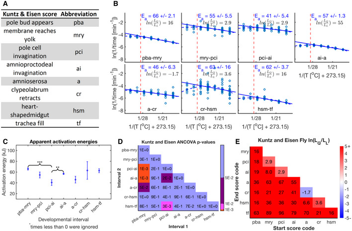
1. Scores Kuntz and Eisen used and abbreviation for the remainder of this figure.

2. Arrhenius plots for durations between adjacent developmental events of Kuntz and Eisen’s data. We fit data for temperatures of 27.5°C and below (dashed red line, i.e., core temperature range) via linear regression (solid blue line). Shown is the apparent activation energy plus/minus the 68% confidence interval. Additionally, we fit the entire temperature range with quadratic (dashed blue line) and linear fits. BIC was also calculated and is shown here as the natural log ratio likelihood for quadratic over linear fit and displayed in black.

3. Apparent activation energies over the core temperature regime are shown. Error bars show the 68% confidence intervals. Black braces point out example developmental intervals that have significantly different apparent activation energies. ‘**’P‐value < 0.01, ‘***’P‐value < 0.001.

4. Shown are P‐values between all developmental intervals. Blue marks P‐values above 5E‐2, purple marks ≤ 5E‐2, pink marks ≤ 1E‐2, and red marks ≤ 1E‐3.

5. Shown are natural log ratio of likelihoods for quadratic over linear fits for all possible developmental intervals, marked by their starting and ending scores, using Kuntz and Eisen’s data over all temperatures. Blue signifies a preference for linearity; red signifies a preference for quadratic behavior.

Figure 3. Fitting the temperature dependence of embryonic development with the Arrhenius equation

1. Example Arrhenius plots for fly embryos for the interval from 14^th Cleavage (A) to Germband Retraction (G) and First Breath (K), respectively. A linear fit (solid black line) and quadratic fit (dashed red line) were fit over all data points (n = 76 & 43 independent biological measurements, respectively). Error bars in temperature represent the standard error (± 0.5°C) of the thermometer used when recording temperature. Error bars in ln(rate) represent standard error. The log ratio of likelihoods for model selection of quadratic over linear is shown in black.

2. Shown are the natural log ratio of (penalized) likelihoods for quadratic over linear model preference, for all fly developmental intervals marked by their starting event (x‐axis) and ending event (y‐axis) (n = 42–84 independent biological measurements). Values above 0 indicate that a quadratic fit is preferred to a linear fit.

3. As (A) but for the frog developmental interval from 3^rd Cleavage (A) to 10^th Cleavage (H) and Late Neurulation (L). Model fits were calculated over all data points (n = 131 and 100 independent biological measurements, respectively).

4. As (B) but for all frog developmental intervals, (n = 97–154 independent biological measurements).

Figure 4. Complexity and non‐idealized behavior of individual enzymes can contribute to non‐idealized behavior of developmental processes

1. Shown is the methodology used to predict the linear regression for fly development from A to G using empirical parameters from individual intervals and equation (3). Far right, this prediction of ln(k) for the composite network (dashed cyan) is overlaid on the empirical data (blue and red error bars) and linear fit (solid black line) for this developmental interval (A–G). Also shown are the color‐coded E_as calculated for each fit over the temperature interval 14.3–27°C (n = 60 independent biological measurements). Error bars in temperature represent the standard error (± 0.5°C) of the thermometer used when recording temperature. Error bars in ln(rate) represent standard error (n = 2–12 biological replicates).

2. Shown is a schematic of a multi‐reaction network from Stage 1 to Stage n. Comparison of two reaction networks modeling equation (3) with 1,000 coupled reactions, one with randomly selected E_a and A (dashed blue line), the second with E_a and A optimized for maximum curvature at 295°K (dashed orange line). To allow direct comparisons, the y‐axes were scaled to result in overlapping tangents calculated at 295°K (solid black line).

3. As (B), however, the worst‐case model (dashed orange) is compared to biological data (blue and red error bars representing standard error in ln(rate), n = 2–12 biological replicates per temperature) from (A). To allow direct comparisons, the y‐axes were scaled to result in overlapping linear fits over 14.3–27°C (solid black line).

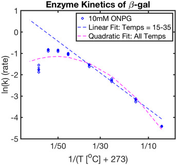
4. Shown is a schematic representing the conversion of NAD+ to NADH via GAPDH catalyzation. GAPDH’s conversion of NAD⁺ to NADH was monitored with UV/VIS spectroscopy at 340 nm. Plotted here is the Arrhenius plot for this conversion at various temperatures between 5°C and 45°C. Means of technical replicates (blue circles) are fit with a linear fit (dashed blue line) from 15 to 35°C and a quadratic fit (dashed magenta) over the entire temperature range. Standard error is shown as blue error bars (n = 2–4 technical replicates per temperature).

Figure EV4. Parameters for linear fits and sequential linear model prediction capture temperature dependence of entire embryonic development well

1. A table showing fly intervals marked by their start and ending scores and their empirically determined prefactors (lnA) and apparent activation energy (E_a) from Fig EV2A.

2. As (A) but for frog prefactors and apparent activation energy calculated empirically from Fig EV2B.

3. Our predictive equation determined in equation (3) for an assumed sequential linear network.

4. Prediction of ln(k) for the composite network (dashed cyan) is overlaid on the empirical data (blue and red error bars) and linear fit (solid black) for this developmental interval (A to K). Also shown are the color‐coded E_as calculated for each fit over the temperature interval 12.2–25.7°C (n = 100 independent biological measurements). Error bars in temperature represent the standard error (± 0.5°C) of the thermometer used when recording temperature. Error bars in ln(rate) represent standard error (n = 2–10 biological replicates per temperature).

Figure EV5. Assay of β‐galactosidase activity over its viable temperature range under 0‐order kinetic conditions

Plotted here is the Arrhenius plot for this conversion. Replicates (blue circles) are fit with a linear fit (dashed blue line) from 15 to 35°C and a quadratic fit (dashed magenta) over the entire viable temperature range. Standard error is shown as blue error bars (n = 3 technical replicates per temperature). Reaction was run using 0.25 U/ml β‐galactosidase.

References

-
- Arcus VL, Mulholland AJ (2020) Temperature, dynamics, and enzyme‐catalyzed reaction rates. Annu Rev Biophys 49: 163–180 - PubMed
- Arcus VL, Prentice EJ, Hobbs JK, Mulholland AJ, Van der Kamp MW, Pudney CR, Parker EJ, Schipper LA (2016) On the temperature dependence of enzyme‐catalyzed rates. Biochemistry 55: 1681–1688 - PubMed
- Arrhenius S (1889) Quantitative relationship between the rate a reaction proceed and its temperature. J Phys Chem 4: 226–248
- Ball DW, Key JA (2014) Intermolecular forces. In Introductory chemistry ‐ 1st Canadian edition, Ball DW, Key JA (eds), pp 531–538. Victoria, BC: BCcampus;
- Begasse ML, Leaver M, Vazquez F, Grill SW, Hyman AA (2015) Temperature dependence of cell division timing accounts for a shift in the thermal limits of C. elegans and C. briggsae . Cell Rep 10: 647–653 - PubMed
Publication types
MeSH terms
Grants and funding
LinkOut - more resources
Full Text Sources
Molecular Biology Databases
Research Materials