The BigBrainWarp toolbox for integration of BigBrain 3D histology with multimodal neuroimaging

Abstract

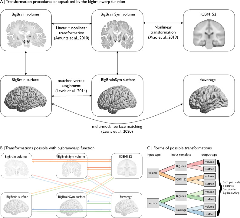
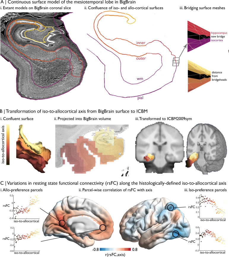
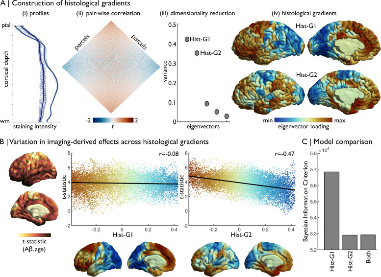
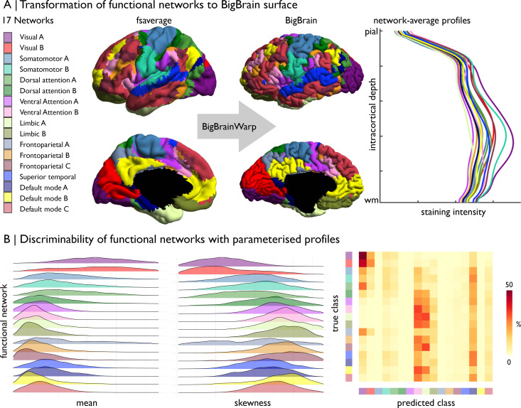
Neuroimaging stands to benefit from emerging ultrahigh-resolution 3D histological atlases of the human brain; the first of which is 'BigBrain'. Here, we review recent methodological advances for the integration of BigBrain with multi-modal neuroimaging and introduce a toolbox, 'BigBrainWarp', that combines these developments. The aim of BigBrainWarp is to simplify workflows and support the adoption of best practices. This is accomplished with a simple wrapper function that allows users to easily map data between BigBrain and standard MRI spaces. The function automatically pulls specialised transformation procedures, based on ongoing research from a wide collaborative network of researchers. Additionally, the toolbox improves accessibility of histological information through dissemination of ready-to-use cytoarchitectural features. Finally, we demonstrate the utility of BigBrainWarp with three tutorials and discuss the potential of the toolbox to support multi-scale investigations of brain organisation.

Keywords: anatomy; histology; human; multi-modal; neuroimaging; neuroscience.

Figure 1.. Magnification of cytoarchitecture using BigBrain, from (A) whole brain 3D reconstruction (taken on https://atlases.ebrains.eu/viewer) to (B) a histological section at 20 µm resolution (available from bigbrainproject.org) to (C) an intracortical staining profile.

The profile represents variations in cellular density and size across cortical depths. Distinctive features of laminar architecture are often observable i.e., a layer IV peak. Note, the presented profile was subjected to smoothing as described in the following section. BigBrainWarp also supports integration of previous research on BigBrain including (D–E) cytoarchitectural and (F–G) morphological models (DeKraker et al., 2019; Paquola et al., 2020a; Paquola et al., 2019; Wagstyl et al., 2020).

Figure 2.. Evaluating BigBrain–MRI transformations.

(A) Volume-based transformations. (i) Jacobian determinant of deformation field shown with a sagittal slice and stratified by lobe. Subcortical+ includes the shape priors (as described in Materials and methods) and the+ connotes hippocampus, which is allocortical. Lobe labels were defined based on assignment of CerebrA atlas labels (Manera et al., 2020) to each lobe. (ii) Sagittal slices illustrate the overlap of native ICBM2009b and transformed subcortical+ labels. (iii) Superior view of anatomical fiducials (Lau et al., 2019). (iv) Violin plots show the Dice coefficient of regional overlap (ii) and landmark misregistration (iii) for the BigBrainSym and Xiao et al., approaches. Higher Dice coefficients shown improved registration of subcortical+ regions with Xiao et al., while distributions of landmark misregistration indicate similar performance for alignment of anatomical fiducials. (B) Surface-based transformations. (i) Inflated BigBrain surface projections and ridgeplots illustrate regional variation in the distortions of the mesh invoked by the modified MSMsulc+ curv pipeline. (ii) Eighteen anatomical landmarks shown on the inflated BigBrain surface (above) and inflated fsaverage (below). BigBrain landmarks were transformed to fsaverage using the modified MSMsulc+ curv pipeline. Accuracy of the transformation was calculated on fsaverage as the geodesic distance between landmarks transformed from BigBrain and the native fsaverage landmarks. (iii) Sulcal depth and curvature maps are shown on inflated BigBrain surface. Violin plots show the improved accuracy of the transformation using the modified MSMsulc+ curv pipeline, compared to a standard MSMsulc approach.

Figure 3.. Overview of spaces and transformations included within BigBrainWarp.

(A) The flow chart illustrates the extant transformation procedures that are wrapped in by the bigbrainwarp function. (B) Arrows indicate the transformations possible using the bigbrainwarp function. The colours, matched to C, reflect distinct functions called within BigBrainWarp. (C) The combination of input type, input template, and output type determines the function called by BigBrainWarp.

Figure 4.. Intrinsic functional connectivity of the iso-to-allocortical axis of the mesiotemporal lobe.

(A) i. BigBrain surface models of the isocortex and hippocampal subfields are projected on a 40 µm resolution coronal slice of BigBrain. (ii–iii) The continuous surface model bridges the inner hippocampal vertices with pial mesiotemporal vertices (entorhinal, parahippocampal or fusiform cortex). Vertices at the medial aspect of the subiculum were identified as bridgeheads and used to bridge between the two surface constructions. Geodesic distance from the nearest bridgehead was used as the iso-to-allocortical axis. (B) Iso-to-allocortical axis values were projected from the surface into the BigBrain volume, then transformed to ICBM2009sym using BigBrainWarp. (C) Intrinsic functional connectivity was calculated between each voxel of the iso-to-allocortical axis and 1000 isocortical parcels. For each parcel, we calculated the product-moment correlation (r) of rsFC strength with iso-to-allocortical axis position. Thus, positive values (red) indicates that rsFC of that isocortical parcel with the mesiotemporal lobe increases along the iso-to-allocortex axis, whereas negative values (blue) indicate decrease in rsFC along the iso-to-allocortex axis.

Figure 5.. Concordance of imaging-derived effects with histological gradients.

(A) Four stages of histological gradient construction. (i) Vertex-wise staining intensity profiles (dotted lines) are averaged within parcels (solid lines). Colours represent different parcels. (ii) Pair-wise partial correlation of parcel-average staining intensity profiles produces a cortex-wide matrix of cytoarchitectural similarity. (iii) The correlation matrix is subjected to dimensionality reduction, in this case diffusion map embedding, to extract the eigenvectors of cytoarchitectural variation. (iv) The eigenvectors capture histological gradients (Hist-G) and are projected onto the BigBrain cortical surface for inspection. (B) The t-statistic cortical map illustrates regional variations in the effect of age on Aβ deposition (Lowe et al., 2019), which was calculated vertex-wise on fsaverage5. To allow comparison, histological gradients were transformed to fsaverage5 using BigBrainWarp. Scatterplots show the association of the t-statistic map with the histological gradients. (C) Bar plot shows the Bayesian Information Criterion of univariate and multivariate regression models, using histological gradients to prediction regional variation in effect of age on Aβ deposition. The univariate Hist-G2 regression had the lowest Bayesian Information Criterion, representing the optimal model of those tested.

Figure 6.. Prediction of functional network by cytoarchitecture.

(A) Surface-based transformation of 17-network functional atlas to the BigBrain surface, operationalised with BigBrainWarp, allows staining intensity profiles to be stratified by functional network. (B) Ridgeplots show the moment-based parameterisation of staining intensity profiles within each functional network. The confusion matrix illustrates the outcome of mutli-class classification of the functional networks, using the central moment of the staining intensity profiles.

Appendix 1—figure 1.. Influence of sampling parameters on staining intensity profiles.

(A) Line plots show how the shape of an exemplar profile is changed by various sampling parameters. Far left is the raw profile constructed with 50 surfaces. Centre left are raw profiles constructed with 50–100 surfaces. Centre right are profiles (constructed with 50 surfaces) and subjected to varied levels of depth-wise smoothing. Far right are profiles (constructed with 50 surfaces and subjected to 10 iterations of depthwise smoothing) with varied levels of surface-wise smoothing. (B) Influence of sampling parameters was evaluated based on spatial autocorrelation and number of peaks. (i–ii) The spatial autocorrelation was defined by the number of steps between two vertices on the mesh, as depicted for an example vertex in (i). Then, we calculated the product-moment correlation between all staining intensity profiles and averaged these values based on the relative distance between vertices. The line plot show a decrease in correlation with increasing distance, attributable to spatial autocorrelation. (iii) The number of peaks was calculated to assess the jaggedness the staining intensity profile. (C) Using the lowest iteration of a sampling parameter as a baseline, we 31 calculated the product-moment correlation of profile features (spatial autocorrelation or number of peaks) with increases in the sampling parameter. In other words, the graph shows the similarity of solutions to the baseline sampling parameters. We found that the surface-wise smoothing impacts the spatial autocorrelation and number of peaks, while the number of surfaces and depthwise smoothing have little-to-no effect on spatial autocorrelation and a small effect on number of peaks. (D) For varying degrees of depth-wise (rows) and surface-wise (columns) smoothing, line plots show spatial autocorrelation and histograms show the distribution of number of peaks across profiles.

References

1. Amunts K, Lepage C, Borgeat L, Mohlberg H, Dickscheid T, Rousseau ME, Bludau S, Bazin PL, Lewis LB, Oros-Peusquens AM, Shah NJ, Lippert T, Zilles K, Evans AC. BigBrain: An Ultrahigh-Resolution 3D Human Brain Model. Science. 2013;340:1472–1475. doi: 10.1126/science.1235381. - DOI - PubMed
1. Amunts K, Zilles K. Architectonic Mapping of the Human Brain beyond Brodmann. Neuron. 2015;88:1086–1107. doi: 10.1016/j.neuron.2015.12.001. - DOI - PubMed
1. Amunts K, Mohlberg H, Bludau S, Zilles K. Julich-Brain: A 3D probabilistic atlas of the human brain’s cytoarchitecture. Science. 2020;4588:1–10. doi: 10.1126/science.abb4588. - DOI - PubMed
1. Arnatkevičiute A, Fulcher BD, Oldham S, Tiego J, Paquola C, Gerring Z, Aquino K, Hawi Z, Johnson B, Ball G, Klein M, Deco G, Franke B, Bellgrove M, Fornito A. Genetic Influences on Hub Connectivity of the Human Connectome. bioRxiv. 2020 doi: 10.1101/2020.06.21.163915. - DOI - PMC - PubMed
1. Avants BB, Epstein CL, Grossman M, Gee JC. Symmetric diffeomorphic image registration with cross-correlation: Evaluating automated labeling of elderly and neurodegenerative brain. Medical Image Analysis. 2008;12:26–41. doi: 10.1016/j.media.2007.06.004. - DOI - PMC - PubMed
Publication types