Technology dictates algorithms: recent developments in read alignment

Abstract

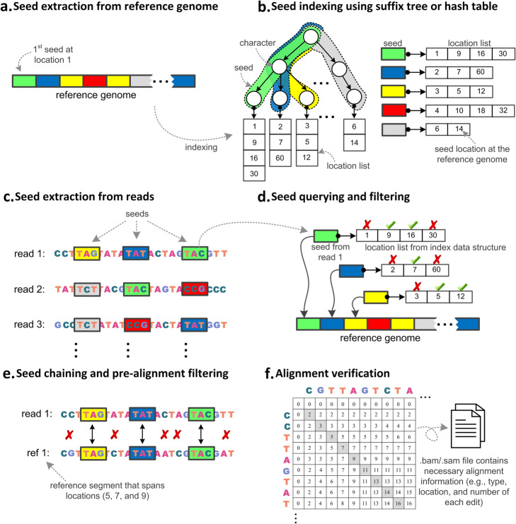
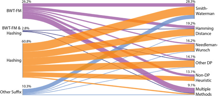
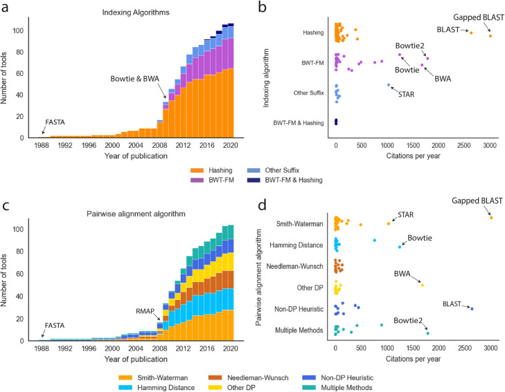
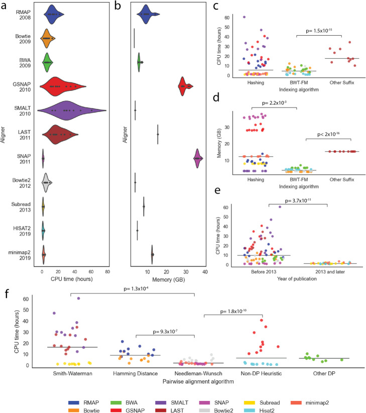
Aligning sequencing reads onto a reference is an essential step of the majority of genomic analysis pipelines. Computational algorithms for read alignment have evolved in accordance with technological advances, leading to today's diverse array of alignment methods. We provide a systematic survey of algorithmic foundations and methodologies across 107 alignment methods, for both short and long reads. We provide a rigorous experimental evaluation of 11 read aligners to demonstrate the effect of these underlying algorithms on speed and efficiency of read alignment. We discuss how general alignment algorithms have been tailored to the specific needs of various domains in biology.

Fig. 1

Overview of a read alignment algorithm. a The seeds from the reference genome sequence are extracted. b Each extracted seed and all its occurrence locations in the reference genome are stored using the data structure of choice (suffix tree and hash table are presented as an example). Common prefixes of the seeds are stored once in the branches of the suffix tree, while the hash table stores each seed individually. c The seeds from each read sequence are extracted. d The occurrences of each extracted seed in the reference genome are determined by querying the index database. In this example, the three seeds from the first read appear adjacent at locations 5, 7, and 9 in the reference genome. Two of the same seeds appear also adjacent at another two locations (12 and 16). Other non-adjacent locations are filtered out (marked with X) as they may not span a good match with the first read. e The adjacent seeds are linked together to form a longer chain of seeds by examining the mismatches between the gaps. Pre-alignment filters can also be applied to quickly decide whether or not the computationally expensive DP calculation is needed. f Once the pre-alignment filter accepts the alignment between a read and a region in the reference genome, then DP-based (or non-DP-based) verification algorithms are used to generate the alignment file (in BAM or SAM formats), which contains alignment information such as the exact number of differences, location of each difference, and their type.

Fig. 2

Combination of algorithms utilized by read alignment tools. Sankey plot displaying the flow of surveyed tools using each indexing technique and pairwise alignment. For every indexing technique, the percentage of surveyed tools using the algorithm is displayed (BWT-FM 26.2%, BWT-FM, and Hashing 2.8%, Hashing 60.8%, Other Suffix 10.3%). For every pairwise alignment technique, the percentage of surveyed tools using the algorithm is displayed (Smith-Waterman 28.3%, Hamming distance 19.2%, Needleman-Wunsch 16.2%, Other DP 14.1%, Non-DP Heuristic 13.1%, Multiple Methods 9.1%)

Fig. 3

The landscape of read alignment algorithms published from 1988 to 2020. a Histogram showing the cumulation of surveyed tools over time colored by the algorithm used for genome indexing. The first published aligner, FASTA, is labeled as well as the point at which Bowtie and BWA were introduced and changed the landscape of aligners. b The popularity of all surveyed aligners, judged by citations per year since the initial release. Tools are grouped by the algorithm used for genome indexing. The six overall most popular aligners are labeled. c Histogram showing the cumulation of surveyed tools over time colored by the algorithm used for pairwise alignment. The two aligners credited to have been the first to use the three most popular algorithms (FASTA: Smith-Waterman and Needleman-Wunsch, RMAP: Hamming distance) are labeled. d The popularity of each surveyed aligner, judged by citations per year since the initial release. Tools are grouped by the algorithm used for pairwise alignment. The six overall most popular aligners are labeled.

Fig. 4

The effect of read alignment algorithms on the speed of alignment and computational resources. Results of the benchmarking performed on 11 surveyed DNA read alignment tools that can be installed through bioconda (RMAP, Bowtie, BWA, GSNAP, SMALT, LAST, SNAP, Bowtie2, Subread, HISAT2, and minimap2) additionally noted in Supplementary Table 2 and Supplementary Note 3. Each tool’s CPU time and RAM required were recorded for 10 different WGS samples from the 1000 Genomes Project. a, b Violin plots showing the relative performance (a CPU time and b RAM) of the benchmarked aligners. Aligners are ordered by year of release. c, d The relative performance (c CPU time and d RAM) of the benchmarked aligners grouped by the algorithm used for genome indexing and colored by individual aligners (BWT-FM CPU time vs. Suffix array CPU time: LRT, p value = 1.5 × 10⁻¹⁵, Hashing memory vs. BWT-FM memory: LRT, p value = 2.2 × 10⁻³, BWT-FM memory vs. Suffix Array memory: LRT, p value < 2 × 10⁻¹⁶). The legend of d is the same for c, e, and f. e The relative performance (CPU time) of the benchmarked aligners grouped by whether the tool was released before or after long-read technology was introduced (2013) and colored by individual aligners (LRT, p value = 3.7 × 10⁻¹¹). f The relative performance (CPU time) of the benchmarked aligners grouped by the algorithm used for pairwise alignment and colored by individual aligners (Needleman-Wunsch CPU time vs. Smith-Waterman CPU time: Wald, p value = 1.3 × 10⁻⁴, Needleman-Wunsch CPU time vs. Hamming Distance CPU time: Wald, p value = 9.3 × 10⁻⁷, Needleman-Wunsch CPU time vs. Non-DP Heuristic CPU time: Wald, p value = 1.8 × 10⁻¹⁰)

References

1. Weissenbach J. The Human Genome. 2002. Human Genome Project: Past, Present, Future; pp. 1–9. - PubMed
1. Shendure J, Ji H. Next-generation DNA sequencing. Nat Biotechnol. 2008;26:1135–1145. doi: 10.1038/nbt1486. - DOI - PubMed
1. Metzker ML. Sequencing technologies — the next generation. Nat Rev Genet. 2009;11:31–46. doi: 10.1038/nrg2626. - DOI - PubMed
1. Payne A, Holmes N, Rakyan V, Loose M. BulkVis: a graphical viewer for Oxford nanopore bulk FAST5 files. Bioinformatics. 2019;35:2193–2198. doi: 10.1093/bioinformatics/bty841. - DOI - PMC - PubMed
1. Goodwin S, McPherson JD, McCombie WR. Coming of age: ten years of next-generation sequencing technologies. Nat Rev Genet. 2016;17:333–351. doi: 10.1038/nrg.2016.49. - DOI - PMC - PubMed
Publication types
LinkOut - more resources