Drosophila re-zero their path integrator at the center of a fictive food patch

Abstract

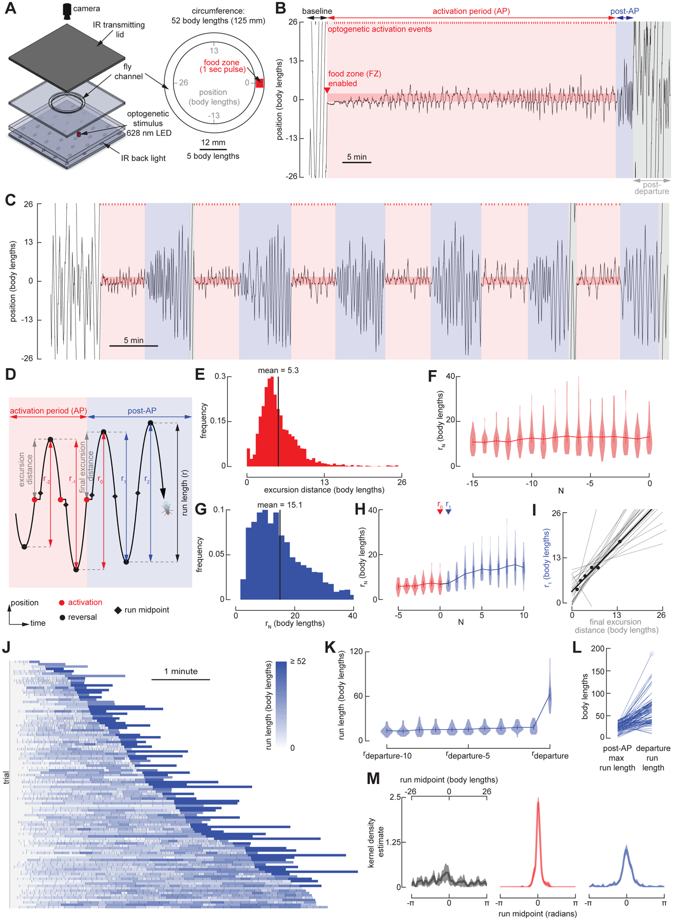
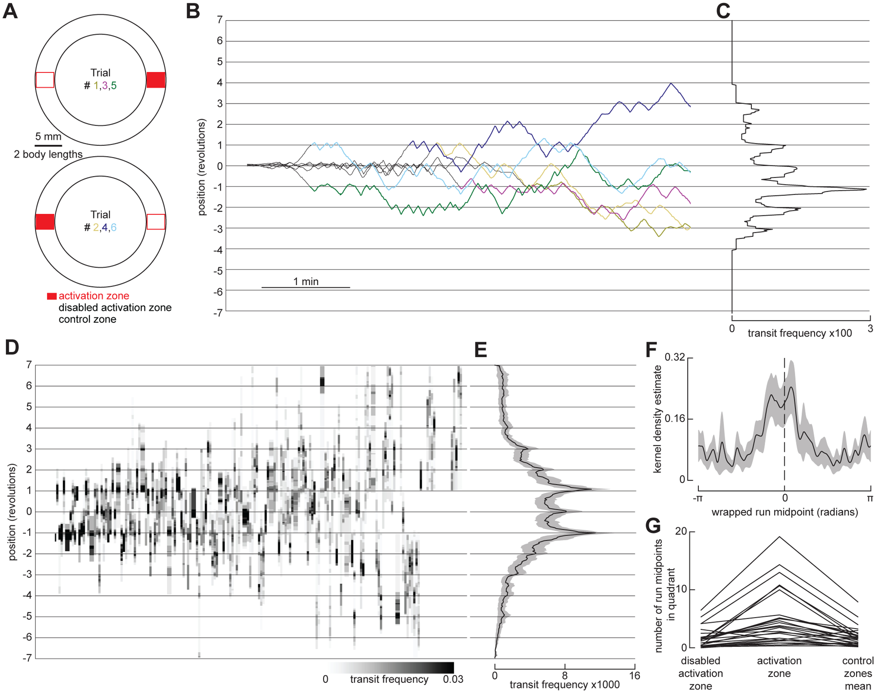
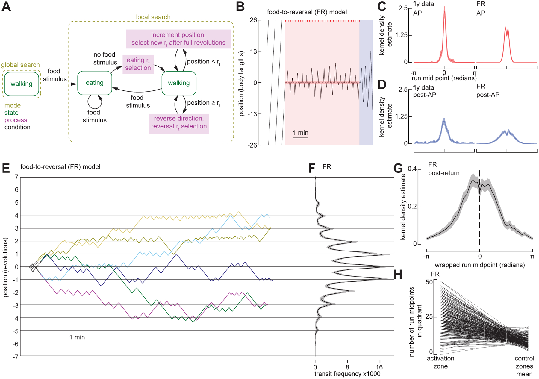
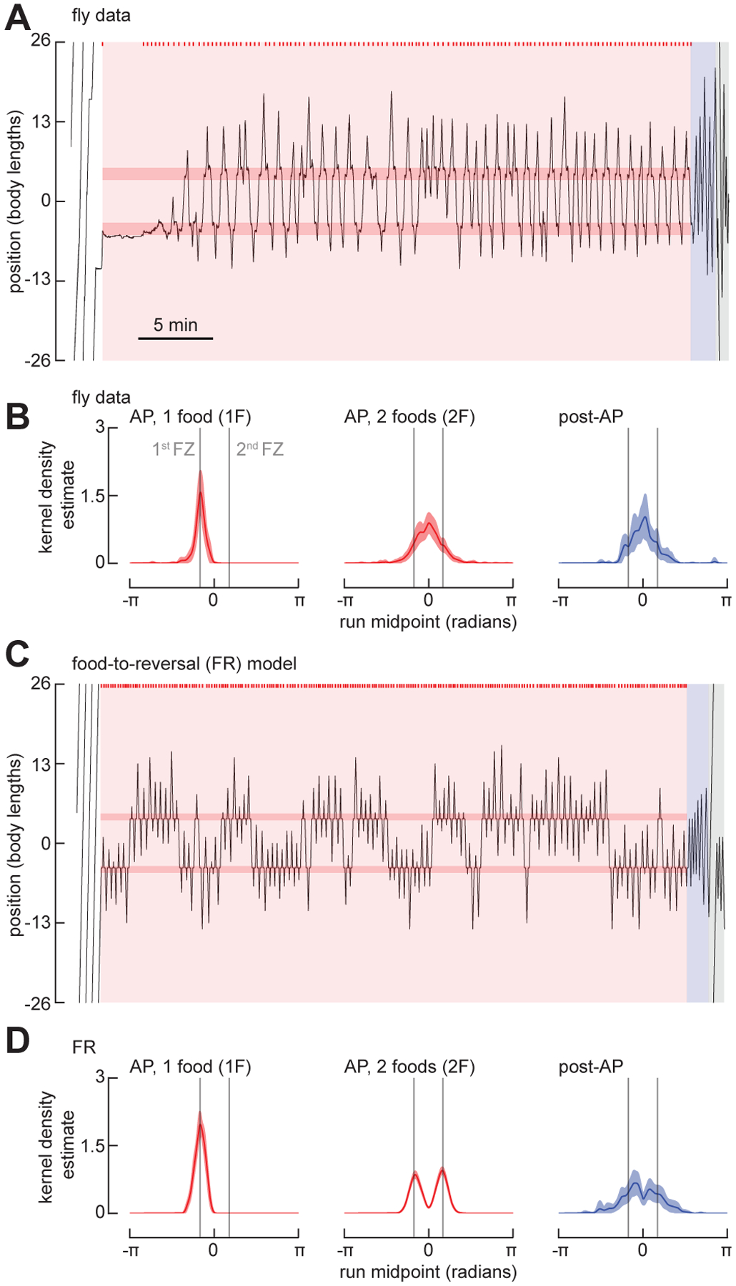
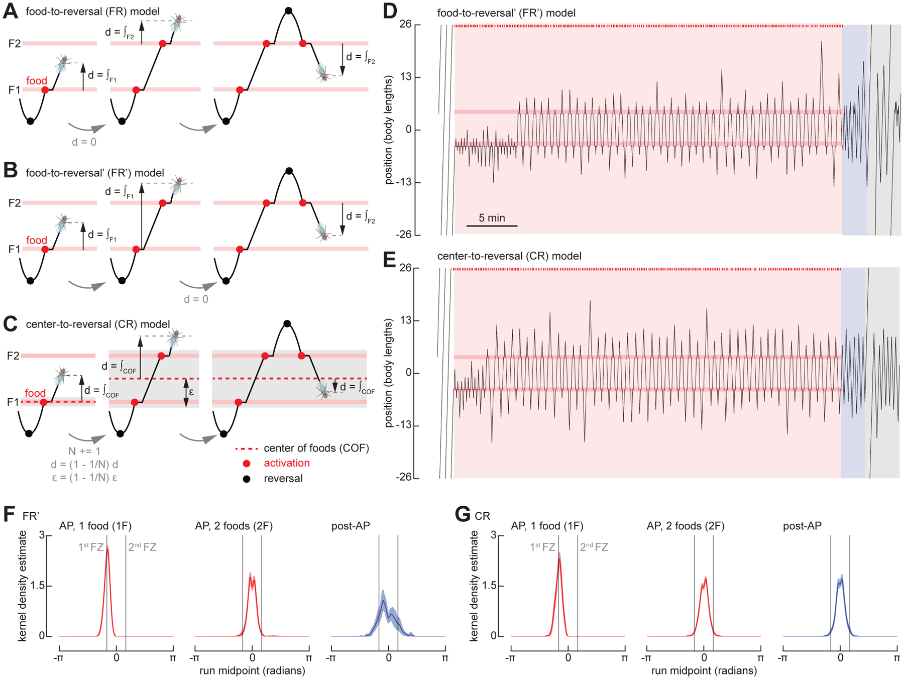
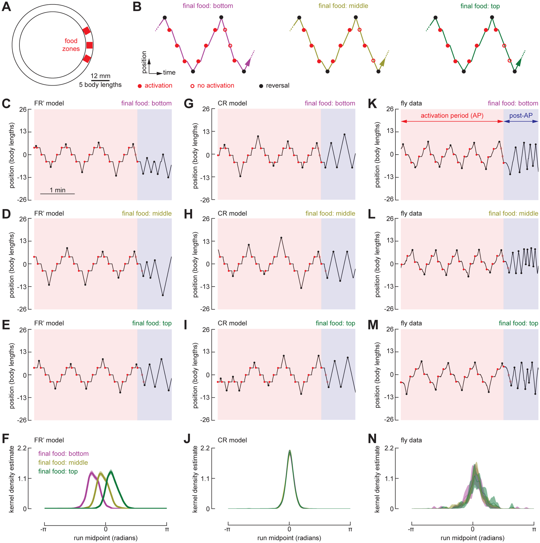
The ability to keep track of one's location in space is a critical behavior for animals navigating to and from a salient location, and its computational basis is now beginning to be unraveled. Here, we tracked flies in a ring-shaped channel as they executed bouts of search triggered by optogenetic activation of sugar receptors. Unlike experiments in open field arenas, which produce highly tortuous search trajectories, our geometrically constrained paradigm enabled us to monitor flies' decisions to move toward or away from the fictive food. Our results suggest that flies use path integration to remember the location of a food site even after it has disappeared, and flies can remember the location of a former food site even after walking around the arena one or more times. To determine the behavioral algorithms underlying Drosophila search, we developed multiple state transition models and found that flies likely accomplish path integration by combining odometry and compass navigation to keep track of their position relative to the fictive food. Our results indicate that whereas flies re-zero their path integrator at food when only one feeding site is present, they adjust their path integrator to a central location between sites when experiencing food at two or more locations. Together, this work provides a simple experimental paradigm and theoretical framework to advance investigations of the neural basis of path integration.

Keywords: Drosophila; odometry; path integration; place memory; state-dependent models.

Figure 1.. Repeated back-and-forth excursions constitute a local search around a fictive food location.

(A) Schematic of the experimental setup (left) and annular arena (right). An overhead camera tracks the position of an individual Gr5a-GAL4>UAS-CsChrimson female fly, in real-time, as it explores a 4 mm-wide circular channel, ~52 body lengths (BL) in circumference. Whenever the fly occupies the featureless food zone, it receives a one-second pulse of optogenetic activation of sugar-sensing neurons via a 628 nm LED positioned beneath the channel, followed by a 15-second refractory period during which the fly cannot receive activation. An infrared (IR) backlight and IR-transmitting lid enable behavioral tracking while otherwise maintaining complete darkness for the fly aside from the brief optogenetic pulses. (B) Example fly trajectory. To simplify the display and analysis of the data, we transformed the curved trajectories of the flies in the circular channel into a wrapped one-dimensional path. This experiment begins with a baseline period, during which the fly does not receive optogenetic activation, followed by a 40-minute activation period (AP, red) during which the optogenetic protocol is operational, followed by a post-activation-period (post-AP, blue) during which the optogenetic protocol is switched off. The post-AP is defined as ending when the fly executes its first run straying more than 26 body lengths (i.e., ½ the arena perimeter) from the food zone, hereafter termed the ‘departure run’. The remaining trajectory is referred to as post-departure (grey). Optogenetic stimulation events during the AP are indicated as red tick-marks (top). See also Figure S1A and Video S1. (C) As in (B), for an experiment with six serial trials each consisting of a 5-minute AP followed by a 5-minute post-AP. See also Figure S1B and Video S1. (D) Schematic, showing features of local search. After encountering a food stimulus during the AP, flies walk a given excursion distance (grey), reverse direction, and perform a run back towards the food. The distance between two consecutive reversals is a run length (r), where r₀ is the run length between the final reversal of the AP and the first reversal of the post-AP, and all other runs are numbered with respect to r₀. The run midpoint is defined as the halfway point between two consecutive reversals. (E) Distribution of all excursion distances, from the 40-min AP experiments as in (B). (N = 29 flies, 2494 food excursions). (F) Run lengths for the final 16 runs of the AP, including r₀, from the 40-min AP experiments. Data from trials with fewer than 16 AP runs are included. (N = 29 flies). Throughout the paper, error bars depict 95% confidence intervals and violin plots indicate full data distributions. (G) Mean distribution of the run lengths of the post-AP from the trial-based experiments as in (C). (N = 22 flies, n = 110 trials). (H) Run lengths for the final 6 runs of the AP, including r₀, and the first 10 runs of the post-AP, from the trial-based experiments as in (C). (N = 22 flies, n = 110 trials). Labels indicate the final run of the AP (r₀) and the first run of the post-AP (r₁). (I) Relationship between the final excursion distance during the AP and the first run of the post-AP (r₁). Black dots indicate r₁ vs. last excursion for 6 trials from the fly in (C), and the black line indicates the linear regression for this fly. Grey lines indicate linear regressions for all remaining flies with data from at least 3 trials. (N = 20 flies). (J) Sequences of post-AP runs and their associated departure run, sorted by the duration of the post-AP. Each row corresponds to a single trial from experiments as in (C), where the length of each box corresponds to the duration of each run, and the color of each box indicates run length. (N = 22 flies, n = 110 trials). Note that in 11 trials at the bottom of the panel, the flies did not execute a departure run before the next AP began. (K) Run lengths for the final 10 runs of the post-AP, as well as the departure run, from data in (J). Data from trials with fewer than 10 post-AP runs are included. (L) Length comparison of the longest post-AP run, and corresponding departure run, for each trial, from data in (J). The 11 trials without a departure run were not included in this analysis. (M) Normalized kernel density estimate (KDE) of the run midpoint in baseline (left), AP (middle), and post-AP (right). (N = 22 flies). Throughout the paper, shaded regions indicate 95% confidence interval. Throughout the paper, the KDE is calculated for each fly for ϰ = 200 and then the mean and 95% confidence interval is calculated for the individual fly’s KDE. For post-AP comparison with simple models, with run lengths randomly drawn from either the empirically derived data shown in Figure 1J (excluding the departure runs), or a Lévy distribution fit to the same data, see Figure S2. See also Video S2 and Video S5.

Figure 2.. Flies reinitiate a local search at a former fictive food site after circling the arena.

(A) Schematic of the smaller annular arena (~26 body lengths), indicating the location of the food zone for each trial, as well as control zones used for analysis. Experiments were done as in Figure 1C, but each food zone was 1.3 body lengths, and the food zone location was alternated from trial to trial. (B) Example pre-return (before the fly has circled the arena at least once during the post-AP, grey) and post-return (colored) trajectories from a single experiment where each line corresponds to a single trial and shows the unwrapped trajectory, with gridlines indicating full revolutions around the arena. To align data for analysis, trajectories from even-numbered trials were shifted such that the location of the food zone is always at 0. See also Video S2. For the model recapitulating fly re-initiation of local search at a former fictive food site after circling the arena, see Figure S4 and Video S5. (C) Mean distribution of fly transits for post-return trajectories in (B). Transits were calculated using bins 2 BL wide and counted when a fly entered a bin from one side and exited the bin from the other side. (D) Heatmap indicating distribution of transits during post-return trajectories, calculated using 4 bins per revolution (dividing the arena into quadrants centered on the food zone, disabled food zone, and each control zone). Each column represents a single trial, with columns sorted by frequency of transits at the 1 or −1 revolution position. (N = 28 flies, n = 168 trials). (E) Mean transit distribution for data in (D). (F) Normalized kernel density estimate (KDE) of the wrapped run midpoint in the post-return period. (N = 28 flies). (G) Number of run midpoints in each arena quadrant during post-return trajectories. (N = 28 flies). Each line shows the values for a single fly, where data from both control quadrants were averaged together.

Figure 3.. An agent-based model using iterative odometric integration recapitulates Drosophila local search around a single fictive food site.

(A) Schematic of the state-transition diagram for an agent-based model. Arrows indicate transitions—governed by conditions—between search modes, behavioral states, and computational processes. For detailed state transition diagrams, including that of the simulated environment, see Figure S3. (B) Example trajectory of FR model simulation in a circular arena with a 52-body length circumference, showing baseline, AP, and post-AP. Plotting conventions as in Figure 1B. (C) Normalized kernel density estimate (KDE) of the run midpoint in during AP for flies (left, N = 22 flies) and FR model (right, N = 300). Data for the fly is re-plotted from Figure 1M. (D) Normalized kernel density estimate (KDE) of the run midpoint in during post-AP for flies (left, N = 22 flies) and FR model (right, N = 300). Data for the fly is re-plotted from Figure 1M. (E) Six representative example trajectories of FR model simulation in a small circular arena with a 26-body length circumference (same as experiments in Figure 2). Plotting conventions as in Figure 2B. (F) Mean transit distribution for FR simulations in small arena. (N = 300). Plotting conventions as in Figure 2E. (G) Normalized kernel density estimate (KDE) of the wrapped run midpoint in the post-return period for FR simulations in small arena. (N = 300). Plotting conventions as in Figure 2F. (H) Number of run midpoints in the food quadrant compared to the other three quadrants during post-return trajectories for FR simulations in small arena. (N = 300). Each line shows the values for a single simulation, where data from all three control quadrants were averaged together.

Figure 4.. The FR model fails to predict Drosophila search behavior around multiple fictive food sites.

(A) Example trajectory of a fly exploring an annular arena with two food zones, spaced 9 body lengths (BL) apart. The experiment consists of a baseline period, AP, and post-AP. Plotting conventions as in Figure 1B. See also Figure S1C and Video S3. For trajectories of flies exploring an annular arena with two food zones, spaced 13 body lengths (BL) apart, see Figure S1D. (B) Normalized KDE of the run midpoint for one-food search (1F, left), the two-food search (trajectory after the fly has encountered the 2^nd food zone, 2F, middle), and the post-AP (right). To align data for analysis for 1F, trajectories for flies that found the food located at +4.5 BL first were shifted such that the first food for all flies is −4.5 BL. (N = 29 flies). (C) As in (A), for a simulation using the FR model. (D) As in (B) for the FR model. The first 300 simulations in which the virtual fly found both food sites are included. (N = 300). See also Video S3.

Figure 5.. Two modified versions of the FR model recapitulate Drosophila search behavior around multiple fictive food sites.

(A) Schematic, showing features of food-to-reversal (FR) model. The virtual fly resets its integrator at each new food that it encounters. (B) As in (A) for food-to-reversal (FR’) model. The virtual fly resets its integrator at the first food encountered after each reversal. (C) As in (A) for center-to-reversal (CR) model. The virtual fly resets its integrator at the center of all the food locations it encounters during a run. (D) As in Figure 4A, for a simulation using the FR’ model. (E) As in Figure 4A, for a simulation using the CR model. See also Video S4. (F) As in Figure 4B, for simulations using the FR’ model. The first 300 simulations in which the virtual fly found both food sites are included. (N = 300). (G) As in Figure 4B, for simulations using the CR model. The first 300 simulations in which the virtual fly found both food sites are included. (N = 300). See also Video S4.

Figure 6.. Flies reset their path integrator at the center of a cluster of fictive food sites.

(A) Schematic of the annular arena with three food zones, spaced 4.5 body lengths apart. (B) Schematic of the experimental paradigm. At the conclusion of the AP, two of the food zones were disabled while one food zone remained capable of providing an additional single optogenetic pulse. For each trial, the final operational food zone was designated to be either the bottom, middle, or top. For trials where the final 3 or more runs during the AP spanned all three food zones, we calculated the KDE of the run midpoint during the post-AP. (C–E) Example trajectories of the FR’ model fly searching across three food zones, in which the final food stimulus is in either the bottom (C), middle (D), or top (E) position. (F) Normalized KDE of the run midpoint in the post-AP period for FR’ model. (N = 300). (G–J) As in (C–F), for simulations using the CR model. (N = 300). (K–N) As in (C–F), for fly data. (N = 45 flies, n = 166 trials).

References

1. Pyke GH (1984). Optimal foraging theory. Annu. Rev. Ecol. Syst 15, 523–575.
1. Whishaw IQ, and Brooks BL (1999). Calibrating space: exploration is important for allothetic and idiothetic navigation. Hippocampus 9, 659–667. - PubMed
1. Wolf H (2011). Odometry and insect navigation. J. Exp. Biol 214, 1629–1641. - PubMed
1. Wehner R, and Müller M (2006). The significance of direct sunlight and polarized skylight in the ant’s celestial system of navigation. Proc. Natl. Acad. Sci 103, 12575–12579. - PMC - PubMed
1. Bühlmann C, Cheng K, and Wehner R (2011). Vector-based and landmark-guided navigation in desert ants inhabiting landmark-free and landmark-rich environments. J. Exp. Biol 214, 2845–2853. - PubMed
Publication types
LinkOut - more resources