Stimulus-dependent representational drift in primary visual cortex

Abstract

To produce consistent sensory perception, neurons must maintain stable representations of sensory input. However, neurons in many regions exhibit progressive drift across days. Longitudinal studies have found stable responses to artificial stimuli across sessions in visual areas, but it is unclear whether this stability extends to naturalistic stimuli. We performed chronic 2-photon imaging of mouse V1 populations to directly compare the representational stability of artificial versus naturalistic visual stimuli over weeks. Responses to gratings were highly stable across sessions. However, neural responses to naturalistic movies exhibited progressive representational drift across sessions. Differential drift was present across cortical layers, in inhibitory interneurons, and could not be explained by differential response strength or higher order stimulus statistics. However, representational drift was accompanied by similar differential changes in local population correlation structure. These results suggest representational stability in V1 is stimulus-dependent and may relate to differences in preexisting circuit architecture of co-tuned neurons.

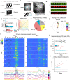
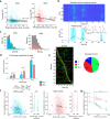
Fig. 1. Chronic 2-photon imaging reveals differential stability of visual responses in single cells.

a Visual stimuli: top screen depicts a drifting grating of one orientation as presented in the passive drifting grating (PDG) stimulus, bottom screen depicts a single frame from the natural movie (MOV) stimulus. PDG is presented first as 8 repeats of a 12 orientation sequence, followed by 30 repeats of MOV. b Location of one example recording field in primary visual cortex (V1). Left: widefield fluorescence image of a 4 mm cortical window for one example Emx1-cre × ROSA-tTA × TITL-GCaMP6s mouse, with overlay (light blue) of visual area boundaries determined by retinotopic mapping (see “Methods”); red box indicates the approximate location of 2-photon recordings in V1; scale bar = 1 mm. Right: example average projection of a 2-photon imaging field; scale bar = 100 μm. Bottom: schematic of the head-fixed mouse. c Example images of registered cells (see “Methods”) from the imaging field in (b) on all recording days. Top row, green: average projection of GCaMP fluorescence channel. Bottom row, red: pixel-wise activity map (see “Methods”). Scale bar = 15 μm. d Top left: single-cell reliability distributions for PDG and MOV stimuli on the first recording session for one example mouse. Reliability is defined as the Pearson correlation coefficient (CC) of trial-averaged activity from two halves of the trials. Middle left: PDG reliability distribution; a subset of PDG responsive neurons is colored. Bottom left: MOV reliability distribution; a subset of MOV responsive neurons is colored. Right: each neuron’s between-trial CC for PDG vs. MOV, for neurons present on the reference session across all mice (n = 4142 neurons). Dots are colored by significant responsiveness to stimuli, as in (e). e Average percentage of neurons significantly responsive to each stimulus (MOV only: 47.7 ± 2.1% sem, PDG only: 9.1 ± 0.9%, both: 20.4 ± 2.3%, none: 22.7 ± 2.2%). f Fluorescence traces (ΔF/F) for one example neuron. Trials are concatenated across sessions. Left: responses to the PDG stimulus; overlay: orientation tuning curves for each recording day. Right: responses to the MOV stimulus. White horizontal lines in each heatmap indicate divisions between recording sessions (8 trials per session for PDG, 30 trials per session for MOV). Heatmaps for each stimulus are co-normalized. Below each heatmap are trial-averaged responses colored by session. g Orientation tuning curves colored by session averaged across all orientation-tuned neurons in all imaging fields and aligned to 0° based on preferred orientation. Neurons are only included if they are present on a given session and orientation tuned (740, 710, 694, 670, 701, 659, 596 neurons per session 1–7 respectively). h Top: representational drift index (RDI) curves for each stimulus for example neuron shown in (f); values closer to 0 indicates a more stable response (similar to the first recording session), and closer to 1 indicates greater response drift (see methods); inset: RDI formula: CC_WS = within-session correlation coefficient, CC_BS = between-session correlation coefficient; dotted line indicates control RDI for this cell, determined using half the trials of the session 1 as the reference and the other half as a test data set (see methods). i Average RDI curves across all imaging fields. Values for each imaging field on a given session are calculated by averaging across neurons that are present on that session and visually responsive to both stimuli. The dotted line indicates control RDI, as in (h). Error bars are ± sem. Significance markers indicate the comparison of average RDI between stimuli for each session (n = 824, 808, 793, 830, 761, 698 neurons from 13, 12, 12, 13, 11, 9 imaging fields for sessions 2–7 respectively; F_1,1648 = 13.0, p = 3.2 × 10⁻⁴, F_1,1616 = 53.0, p = 5.2 × 10⁻¹³, F_1,1586 = 23.9, p = 1.1 × 10⁻⁶, F_1,1660 = 12.9, p = 3.4 × 10⁻⁴, F_1,1522 = 19.9, p = 8.6 × 10⁻⁶, F_1,1396 = 8.0, p = 4.8 × 10⁻³ for sessions 2–7 respectively; two-tailed F-test using a linear mixed-effects model, fixed effect for stimulus, random effect for mouse; **p < 0.01, ***p < 0.001).

Fig. 2. Characterization of dynamic response events underlying single-cell responses.

a Single neuron RDI as a function of responsiveness (session-average z-score of ΔF/F activity). Each colored dot is one neuron; black dots are 10th percentile binned means; black line is a linear fit of the binned data; shaded area indicates 95th percent confidence interval of the linear fit. Neurons are z-scored using the entire recording on a given session. Data are shown for all neurons responsive to both PDG and MOV (n = 736 neurons). b Response events from one example neuron. Top: ΔF/F responses, all trials across all recording sessions. Bottom: Trial-averaged response. Shaded areas indicate identified events. Insets: z-score trajectories (smoothed using 30-point moving average) across all trials for the three events in the example neuron. c Number of response events per neuron. Left: all PDG responsive neurons are shown in gray, dual-responsive neurons shown in color. Right: all MOV responsive neurons shown in gray, dual-responsive neurons shown in color. d Proportions of event types (growing, decaying, and static) in responses to both stimuli. Event type is determined by z-scoring an event waveform’s single-trial responses and comparing the distributions of these values between the first two sessions (60 trials) and the last two sessions (60 trials; Wilcoxon rank-sum test). Gray dots are individual fields. Bar data shown are mean proportions across all imaging fields ± sem (n = 13 imaging fields; growing events t₁₂ = −2.6, p = 0.04; decaying events t₁₂ = −4.2, p = 0.001; static events t₁₂ = 4.8, p = 3.8 × 10⁻⁴; two-tailed paired-samples t-test; *p < 0.05, **p < 0.01, ***p < 0.001). e Visualization of MOV response event magnitude changes. Left: bands indicate event periods for each neuron, colored by event type. Neurons are ordered by time of maximum trial-averaged response. Right: proportions of event types for neurons’ peak responses (diagonal of the left plot). Data are shown for all dual-responsive neurons. f Event instability (normalized delta z-score) as a function of event magnitude (session-average event z-score). Each colored dot is one event; black dots are 10th percentile binned means ± 95th percent confidence interval. Box plots are the first quartile of data tested against the fourth quartile (n = 365 events per quartile for PDG, Z = 7.3; n = 441 events per quartile for MOV, Z = 3.4; ***p < 0.001, two-sided Wilcoxon ranksum test). Data are shown for all dual-responsive neurons. Boxplots are centered on the median, boxes extend to first and third quartiles, whiskers extend to 1.5 times the interquartile range or minima/maxima in the absence of outliers. g MOV events are less stable than PDG events independent of event magnitude. Binned means (10th percentiles) using data from (f) for both stimuli shown together. Data from all events across both stimuli were pooled to determine bin edges, events from each stimulus were then binned separately. Error bars represent the 95th percent confidence interval, gray lines are linear fits of the data. Significance markers indicate comparison of PDG and MOV values in each bin (**p < 0.01 for first bin, ***p < 0.001 for all other bins; two-sided Wilcoxon rank-sum test).

Fig. 3. Translaminar imaging shows equal RDI distributions across layers.

a Schematic of glass microprism placement in V1. The red dotted line depicts the translaminar imaging plane, which is rotated 90° from the original horizontal plane and spans ~700 μm of the cortical column, capturing neurons in L2-5 for a typical recording. b Example average fluorescence image from a chronic imaging session of a prism field. Colored boxes are zoomed-in example cells (red: L2/3 pyramidal neuron, green: L4 stellate neuron, blue: L5 pyramidal neuron). Scale bar = 100μm. c Delineation of cortical layers. Left: ROI density of binned pixel windows perpendicular to the cortical column axis (corresponds to right subfigure); layers are determined by finding peak density and assigning a 140 μm window around it as L4, and then a further 150 μm from the L4 deep boundary as L5. Right: example field is shown in (b) with an overlay of all ROIs colored by layer; dotted line is the translaminar axis. d Example field shown in (b, c) with an overlay of ROIs of all well-tracked neurons responsive to MOV, colored according to MOV RDI. Dotted lines are layer boundaries. e Session-averaged RDI distributions by stimulus and layer, using all dual-responsive neurons recorded in prism fields (n = 64 L2/3 neurons, 111 L4 neurons, 121 L5 neurons from 4 mice). No significant difference was found between layers, a significant difference was found between stimuli (layer F_2,588 = 2.06, p = 0.12; stimulus F_1,588 = 45.7, p = 3.32 × 10⁻¹¹; two-way ANOVA). Dotted lines indicate control RDI (as in Fig. 1h, i) using all dual-responsive neurons. Boxplots are centered on the median, boxes extend to first and third quartiles, whiskers extend to 1.5 times the interquartile range or minima/maxima in the absence of outliers.

Fig. 4. Inhibitory neuron populations also exhibit representational drift to MOV stimuli.

a Average fluorescence image from an example field of inhibitory neurons in L2/3 of V1 of GAD2-Cre × TITL2-G6s mice. Scale bar = 100 μm. b Example images of well-tracked neurons (see “Methods”) from the field in (a) on all recording days, green and red colors are the same as in Fig. 1c. Scale bar = 15 μm. c Fluorescence traces (ΔF/F) for one example neuron. Trials are concatenated across sessions. Left: responses to PDG. Right: responses to MOV. White horizontal lines indicate divisions between recording sessions. Heatmaps for each stimulus are co-normalized. Below each heatmap are trial-averaged responses colored by session. d Average percentage of neurons responsive to each stimulus (MOV only: 59.4 ± 1.9% sem, PDG only: 0.6 ± 0.6%, both: 14.4 ± 5.7%, none: 25.6 ± 6.3%). e RDI curves for the example neuron shown in (c); dotted line indicates control RDI for this cell (see “Methods”). f Average RDI curves from neurons across all imaging fields; error bars are ± sem; data shown for dual-responsive neurons present on any given session (n = 33, 34, 34, 33, 33, 31 neurons from 4 fields for sessions 2–7 respectively); significance markers indicate the comparison of each session’s PDG RDI values and MOV RDI values (F_1,64  = 0.6, p = 0.44, F_1,66 = 0.3, p = 0.61, F_1,66 = 6.6, p = 0.01, F_1,64 = 5.6, p = 0.02, F_1,64 = 7.9, p = 0.007, F_1,60 = 15.1, p = 2.5 × 10⁻⁴ for sessions 2–7 respectively; two-tailed F-test using a linear mixed-effects model, fixed effect for stimulus, random effect for mouse; *p < 0.05, **p < 0.01, ***p < 0.001). Dotted lines indicate control RDI as in previous figures.

Fig. 5. Stability is not dependent on the higher-order statistics of the visual stimulus.

a Visual stimuli, where the original 30 repeats of MOV is replaced with 20 repeats each of 0%, 50, and 100% phase-scrambled versions of the original movie, randomly interleaved. Bottom screens depict the same freeze-frame from each of the movie versions. b Average RDI curves from all imaging fields; error bars are ± sem; values are calculated using only neurons that are present on any given session (n = 120, 118, 118, 119, 113, 111 neurons from 3 fields for sessions 2–7 respectively). Average PDG RDI is significantly different from average MOV RDI for all three movie versions (0% scramble F_1,380 = 10.7, p = 0.001, F_1,368 = 6.6, p = 0.01, F_1,378 = 40.2, p = 6.6 × 10⁻¹⁰, F_1,374 = 4.9, p = 0.03, F_1,362 = 8.1, p = 0.005, F_1,344 = 4.9, p = 0.03 for sessions 2–7 respectively; 50% scramble F_1,380 = 52.7, p = 2.2 × 10⁻¹², F_1,368 = 7.4, p = 0.007, F_1,378 = 24.7, p = 1.0 × 10⁻⁶, F_1,374 = 4.2, p = 0.04, F_1,362 = 5.3, p = 0.02, F_1,344 = 2.9, p = 0.09 for sessions 2–7 respectively; 100% scramble F_1,380 = 26.8, p = 3.6 × 10⁻⁷, F_1,368 = 9.4, p = 0.002, F_1,378 = 27.9, p = 2.1 × 10⁻⁷, F_1,374 = 5.9, p = 0.02, F_1,362 = 9.3, p = 0.002, F_1,344 = 6.5, p = 0.01 for sessions 2–7 respectively; two-tailed F-test using a linear mixed-effects model, fixed effect for stimulus, random effect for mouse; *p < 0.05, **p < 0.01, ***p < 0.001; color of asterisk corresponds to MOV stimulus version compared to PDG). Dotted lines indicate control RDI, as in previous figures.

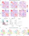
Fig. 6. Between-neuron signal correlation stability is stimulus-dependent.

a Pairwise signal correlations on session 1 (left), final session (middle), and their difference (right) for one example field. Neurons are sorted by the time of peak response on D₀ for each stimulus. Data are shown for all neurons responsive to both stimuli. b Distributions of the single-neuron average change in signal correlations between first and final sessions for example field in A. Dotted lines are means for each stimulus (n = 66 neurons, Z = 2.3, p = 0.02, two-sided Wilcoxon rank-sum test; *p < 0.05). c Field-average changes in signal correlation between first and final sessions. Data shown for all fields. (n = 13 imaging fields; t₁₂ = 3.8, p = 0.003, two-tailed paired-sample t-test; **p < 0.01). d Average instability of signal correlation matrices with respect to the first session over time (1 − CC_BS; where CC_BS is the 2D cross-correlation between signal correlation matrices). Data shown for all fields. Error bars are ± sem; significance markers indicate comparison of PDG and MOV values on the given session (n = 13, 12, 12, 13, 11, 9 imaging fields for sessions 2–7 respectively; t₁₂ = 2.2, p = 0.04, t₁₁ = 5.8, p = 1.2 × 10⁻⁴, t₁₁ = 6.9, p = 2.4 × 10⁻⁵, t₁₂ = 5.0, p = 3.1 × 10⁻⁴, t₁₀ = 4.5, p = 0.001, t₈ = 3.4, p = 0.009, for sessions 2–7 respectively, two-tailed paired-sample t-test; *p < 0.05, **p < 0.01, ***p < 0.001). e Schematic depicting the relationship between stimulus tuning stability and shifts in functional connectivity over time.

References

1. Chklovskii DB, Mel BW, Svoboda K. Cortical rewiring and information storage. Nature. 2004;431:583–618. - PubMed
1. Holtmaat A, Svoboda K. Experience-dependent structural synaptic plasticity in the mammalian brain. Nat. Rev. Neurosci. 2009;10:647–658. - PubMed
1. Lee CR, Najafizadeh L, Margolis DJ. Investigating learning-related neural circuitry with chronic in vivo optical imaging. Brain Struct. Funct. 2020;225:467–480. - PMC - PubMed
1. Dhawale AK, et al. Automated long-term recording and analysis of neural activity in behaving animals. Elife. 2017;6:1–40. - PMC - PubMed
1. Stevenson IH, et al. Statistical assessment of the stability of neural movement representations. J. Neurophysiol. 2011;106:764–774. - PMC - PubMed
Publication types