Task-Driven Learned Hyperspectral Data Reduction Using End-to-End Supervised Deep Learning

Abstract

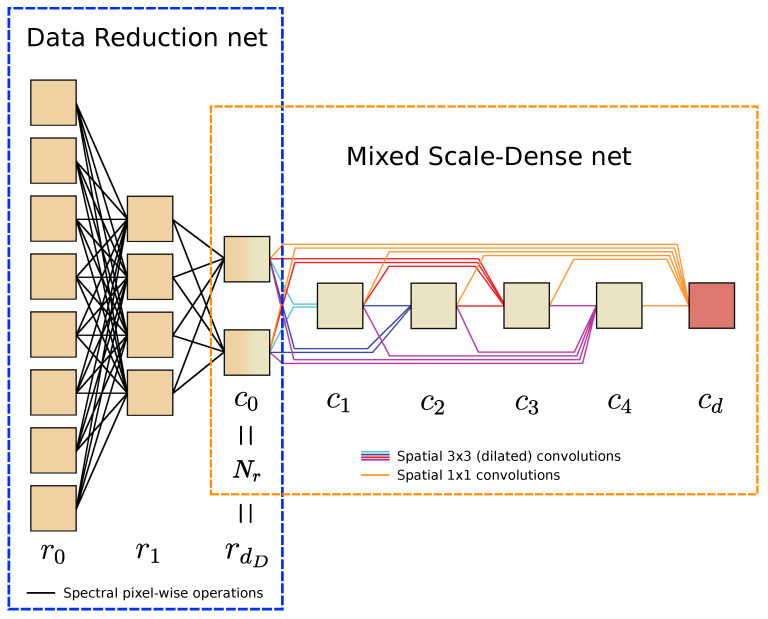
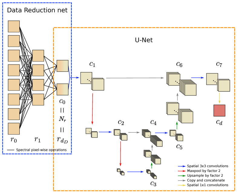
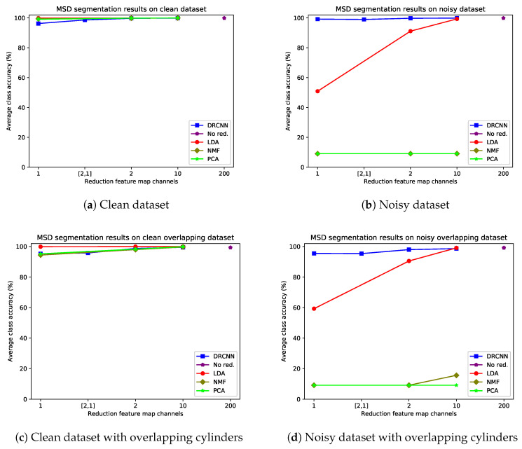
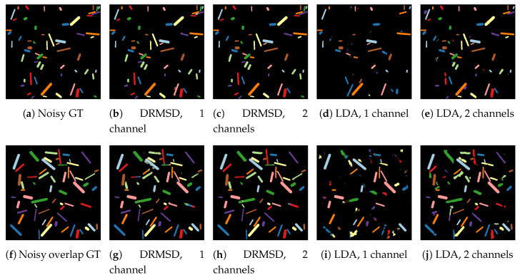
An important challenge in hyperspectral imaging tasks is to cope with the large number of spectral bins. Common spectral data reduction methods do not take prior knowledge about the task into account. Consequently, sparsely occurring features that may be essential for the imaging task may not be preserved in the data reduction step. Convolutional neural network (CNN) approaches are capable of learning the specific features relevant to the particular imaging task, but applying them directly to the spectral input data is constrained by the computational efficiency. We propose a novel supervised deep learning approach for combining data reduction and image analysis in an end-to-end architecture. In our approach, the neural network component that performs the reduction is trained such that image features most relevant for the task are preserved in the reduction step. Results for two convolutional neural network architectures and two types of generated datasets show that the proposed Data Reduction CNN (DRCNN) approach can produce more accurate results than existing popular data reduction methods, and can be used in a wide range of problem settings. The integration of knowledge about the task allows for more image compression and higher accuracies compared to standard data reduction methods.

Keywords: compression; convolutional neural network; deep learning; feature extraction; hyperspectral imaging; machine learning; segmentation.

Figure 1

Schematic architecture of a neural network for image processing. Squares denote feature map channels and arrows denote function inputs. The depth of the network is given by d.

Figure 2

Schematic architecture of a neural network with dependencies between all layers. Squares denote feature map channels and arrows denote function inputs. The network depth is given by d.

Figure 3

Schematic structure of a Data Reduction CNN example. The entire setup consists of a CNN of choice, for example with down- and upscaling layers as shown here, and a data reduction subnetwork in front. This subnetwork repeatedly decreases the number of images from $r_0$ down to $r_{d_D}$ by taking linear combinations of the input images. After that, the CNN carries out the segmentation task.

Figure 4

Example of a Data Reduction Mixed-Scale Dense (MSD) network structure. The number of channels are indicated with the feature maps. Since $w=1$ is chosen, $c_i=1$ for $i>0$. The data are reduced from $r_0=8$ input images to $r_{d_D}=N_r=c_0=2$ feature map channels in the data reduction net, while the segmentation task is performed by an MSD net of depth $d=5$. Each $3\times 3$ convolution is followed by a Rectified Linear Unit (ReLU) operation.

Figure 5

Example of a Data Reduction U-Net structure. The number of channels are indicated with the feature maps. The data are reduced from $r_0=8$ input images to $r_{d_D}=N_r=c_0=2$ feature map channels in the data reduction net. Each $3\times 3$ convolution is followed by a ReLU operation. The number of channels is shown after each convolution and concatenation operations. The network is designed to have $c_1=c_7$, $c_2=c_5=2c_1$, $c_3=4c_1$, $c_4=6c_1$ and $c_6=3c_1$. The value of $c_d$ is equal to the number of segmentation classes $\left|\mathcal{C}\right|$.

Figure 6

Schematic overview of the hyperspectral X-ray projection setup with a cone beam geometry.

Figure 7

Example of the simulated material projections before material designation. The cylinders are shown to be all combined in one image (a), and separately (b).

Figure 8

Mass attenuation spectra for zinc, silver, cadmium, actinium and polyethylene from 6 keV to 71 keV (a). In this spectral region, zinc, cadmium and actinium have one K-edge, polyethylene has none, while actinium has multiple edges. Note that the K-edges of silver and cadmium are relatively close to each other. This holds for all adjacent atomic numbers (not shown in this figure). (b) The normalized plot of the source spectrum ${\overline{I}}_0$ used for generating the hyperspectral X-ray projections.

Figure 9

Visualization of the simulated X-ray data at different bins. The K-edge transition of cadmium is visible between bins 65 and 75 (among (a)–(d), compare (b,c) for example). The data in bins 1 and 300 (e,h) are much more noisy than in bins 65 and 75 (f,g), due to low source spectrum values at bin 1 and 300.

Figure 10

Reflectance spectra used for this dataset (a). The 10 target spectra on the right (b) are a subset of the 60 spectra. The filenames of these target spectra in the USGS Library are added.

Figure 11

The solar irradiance spectrum used for the remote sensing experiments. Note that the drops to a value close to 0 in the graph, particularly at wavelengths 1350–1400 nm and 1800–1950 nm, are mostly due to absorption by water vapor.

Figure 12

Visualization of the simulated remote sensing data. The clean data and the ground truth are shown in (a,b), respectively. When the described Gaussian noise is added to this data, many bins still resemble the clean data, but (c) shows a moderately noisy bin and (d) shows an extremely noisy bin, resulting from differences in solar irradiance. The data with overlapping cylinders and their representation as ground truths are given in (e,f).

Figure 13

Average class accuracies for different data reduction methods using MSD (a) and U-Net (b) on the noisy multi-material X-ray dataset. As a reference, the results for standard MSD and U-Net net are included, which act directly on all 300 spectral bins.

Figure 14

Average class accuracies for different reduction schemes with MSD as CNN for different simulated remote sensing datasets: clean dataset (a), noisy dataset (b), clean overlapping dataset (c) and noisy overlapping dataset (d). The layered reductions to 2 and then 1 feature map channel(s) are indicated by $[2,1]$.

Figure 15

Average class accuracies for different reduction schemes with U-Net as CNN for different simulated remote sensing datasets: clean dataset (a), noisy dataset (b), clean overlapping dataset (c) and noisy overlapping dataset (d). The layered reduction to 2 and then 1 feature map channel(s) is indicated by $[2,1]$.

Figure 16

Visual results for LDA and DRMSD reduction schemes for reductions to 1 and 2 feature map channels on the noisy dataset (a–e) and the noisy overlapping dataset (f–j).

Figure 17

Visual comparison of the data reduction methods for reduction of the noisy many material dataset (a,b) to 1 image. Despite the high noise, DRMSD (c) and DRUNet (d) create the most distinctive images with respect to the ground truth (note the dark shapes at the target cylinder locations, indicated by red circles). The PCA (e) and LDA (f) compressions are included, but the Nonnegative Matrix Factorization (NMF) compression is omitted, as it is highly similar to the PCA compression.

Figure 18

Data reduction weights per bin after training with DRMSD (a) and DRUNet (b) on the noisy few-material X-ray dataset. The K-edge of the material of the objects to be detected (silver) is located between bins 63 and 64 (indicated in orange), which is the location of the drop. The K-edge of cadmium is indicated in green. Additionally, note that the absolute value of the weights decreases when approaching bin 1 or 300.

Figure 19

Example of data reduction weights (d,e) and resulting compressions (compare with ground truth (a)) for DRMSD (b) and DRMSD (c) with reduction to one feature map channel for the noisy remote dataset without overlap.

References

1. Elmasry G., Kamruzzaman M., Sun D.W., Allen P. Principles and applications of hyperspectral imaging in quality evaluation of agro-food products: A review. Crit. Rev. Food Sci. Nutr. 2012;52:999–1023. doi: 10.1080/10408398.2010.543495. - DOI - PubMed
1. Makantasis K., Karantzalos K., Doulamis A., Doulamis N. Deep supervised learning for hyperspectral data classification through convolutional neural networks; Proceedings of the 2015 IEEE International Geoscience and Remote Sensing Symposium (IGARSS); Milan, Italy. 26–31 July 2015; pp. 4959–4962.
1. Habermann M., Frémont V., Shiguemori E.H. Feature selection for hyperspectral images using single-layer neural networks; Proceedings of the 8th International Conference of Pattern Recognition Systems (ICPRS 2017); Madrid, Spain. 11–13 July 2017; pp. 1–6.
1. Chang C.I. Hyperspectral Data Processing: Algorithm Design and Analysis. John Wiley & Sons; Hoboken, NJ, USA: 2013.
1. Lu G., Fei B. Medical hyperspectral imaging: A review. J. Biomed. Opt. 2014;19:010901. doi: 10.1117/1.JBO.19.1.010901. - DOI - PMC - PubMed
LinkOut - more resources