What is the dynamical regime of cerebral cortex?

Abstract

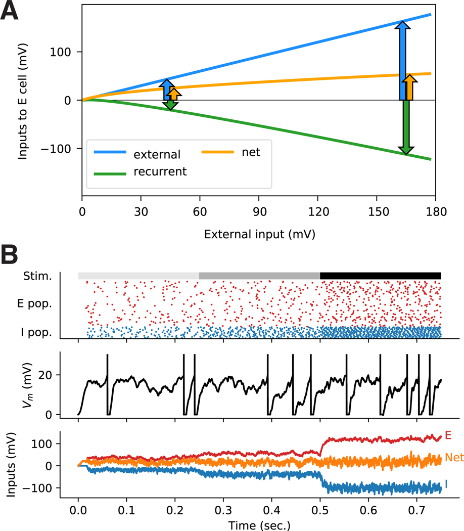
Many studies have shown that the excitation and inhibition received by cortical neurons remain roughly balanced across many conditions. A key question for understanding the dynamical regime of cortex is the nature of this balancing. Theorists have shown that network dynamics can yield systematic cancellation of most of a neuron's excitatory input by inhibition. We review a wide range of evidence pointing to this cancellation occurring in a regime in which the balance is loose, meaning that the net input remaining after cancellation of excitation and inhibition is comparable in size with the factors that cancel, rather than tight, meaning that the net input is very small relative to the canceling factors. This choice of regime has important implications for cortical functional responses, as we describe: loose balance, but not tight balance, can yield many nonlinear population behaviors seen in sensory cortical neurons, allow the presence of correlated variability, and yield decrease of that variability with increasing external stimulus drive as observed across multiple cortical areas.

Figure 1:. Balance of excitation and inhibition.

A: a neuron receiving K_E excitatory and K_I inhibitory recurrent inputs with unitary strengths J_E and J_i, respectively, and K_X excitatory external inputs with unitary strength J_X. B: Top: Spike rasters from a simulation of a network of spiking integrate-and-fire neurons in the asynchronous irregular regime. Spike trains of representative subpopulations of excitatory (red) and inhibitory (blue) cells are shown. The external input to the network is turned on at t = 0. Middle: The membrane voltage trajectory of a typical excitatory neuron in the network. Bottom: Inputs to the same neuron over time: recurrent excitatory (E) and external excitatory (X) inputs, which together provide the total excitatory input (red); inhibitory input (I, blue); and net inputs (yellow). The arrows show the steady-state means (μ) and standard deviations (σ) of the excitatory, inhibitory, and net inputs. The horizontal gray lines in middle and bottom plots show the spiking threshold. This network is in a regime of tight balance of excitation and inhibition: the net input, after cancellation of excitatory and inhibitory inputs, is much smaller than the factors that cancel.

Figure 2:. The supralinear (power-law) neuronal transfer function.

The transfer function of neurons in cat V1 is non-saturating in the natural dynamic range of their inputs and outputs, and is well fit by a supralinear rectified power-law with exponents empirically found to be in the range 2–5. Such a curve exhibits increasing input-output gain (i.e. slope, indicated by red lines) with growing inputs, or equivalently with increasing output firing rates. Gray points indicate a studied neuron’s average membrane potential and firing rate in 30ms bins; blue points are averages for different voltage bins; and black line is fit of power law, $r={[V-\theta ]}_{+}^p$, where r is firing rate, V is voltage, ${[x]}_{+}=x,x>0,=0$ otherwise; θ is a fitted threshold; and p, the fitted exponent, here is 2.79. Note that this shows that firing rate depends supralinearly on mean voltage, but the loosely balanced circuits described here rely on rate depending supralinearly on $\mathbf{u}=\mathbf{W}{\mathit{r}}^{\ast }+\mathbf{I}$. The voltage may be sublinear in this quantity, due to synaptic depression of the recurrent inputs, spike-rate adaptation, post-spike reset, or input-induced conductance increases; it may be supralinear in this quantity, due to synaptic facilitation of recurrent inputs or dendritic excitability. The models rely on the assumption that any sublinearity in the net transformation from u to voltage is insufficient to undo the supralinear voltage-to-firing-rate transformation, yielding a net supralinear transformation from u to firing rate. Figure modified from Priebe et al. (2004).

Figure 3:. Loose vs. tight balance.

A. Simulation of a rate model, the Stabilized Supralinear Network (SSN). The plot shows the external input (blue), the recurrent or within-network input (green), and the net input (orange, equal to external plus recurrent) to the excitatory cell receiving the peak stimulus. At all biological ranges of external input (stimulus) strength, the balance is loose, as exhibited by the left set of three arrows (representing the external, recurrent, and net inputs): the net input is comparable in size to the other two. The balance systematically tightens with increasing external input (right set of arrows), as the net input grows only sublinearly with increasing external input strength. At high (possibly non-biological) levels of external input, the balance will become tight, with the net input much smaller in magnitude than the external and recurrent inputs. The neurons were arranged in a ring topology (there was an E/I neuronal pair at each position on the ring), with position on the ring corresponding e.g. to preferred direction, as in (Ahmadian et al., 2013; Rubin et al., 2015). The strength of synaptic connections decreased with distance over the ring, and external (stimulus-driven) input peaked at the stimulus direction. B. Simulations of a randomly-connected network of N_E = 9600 excitatory and N_I = 2400 inhibitory integrate-and-fire spiking neurons, in the asynchronous irregular regime, receiving increasing levels of external input. The network had ring topology, as in A, with probability rather than strength of connections decreasing with distance, Top: spike rasters of 80 excitatory and 20 inhibitory neurons (randomly chosen from the portion of the ring approximately tuned to the stimulus). The gray bars on top denote the three stages with different levels of external input, μ_X, which for the stimulus-tuned neurons were at 0.5, 1.5 and 4, in units of the rest-to-threshold distance (which was 20 mV), respectively (other key parameters: ${\sigma }_X=0.2$ in same units, all K_AB = 480 on average, and for existing connections $J_{\text{EE}}=0.63\text{mV}$, $J_{\text{IE}}=0.6\text{mV}$, $J_{\text{EI}}=0.32\text{mV}$, $J_{\text{II}}=0.25\text{mV}$). Middle: voltage trace of a randomly chosen E cell from the subpopulation shown in the top rasters. Bottom: E, I, and net input to the same cell. The balance tightens with growing external input strength; in the first two stages (up to t = 0.5 s) the network is in a loose balance regime $(0.1<\beta <1)$, while in the last stage $(t<0.5s)$ it is tightly balanced $(\beta <0.1)$.

Figure 4:. Nonlinear neural behaviors in the loosely balanced regime.

All panels are based on simulations of a Stabilized Supralinear Network (SSN). A,B: same ring model as in Fig. 3A. A) Three forms of response summation, for three levels of input (indicated by colors, corresponding to arrows in B): supralinear summation, for very weak stimuli (left); sublinear summation, for stronger stimuli yielding loose balance (middle); and approximately linear summation, for very strong stimuli yielding tight balance (right). The x-axis is position on the ring, unrolled into a line. Black line shows profile of responses across excitatory population to a 90° stimulus; response to a 270° stimulus is identical except shifted to peak at 270°. Green dotted lines show linear sum of responses to these two stimuli. Red lines show actual responses when the two stimuli are presented simultaneously. B): Additivity index is height of peak response to the two stimuli together (red lines in A), divided by peak height of the linear summation of responses to each stimulus (green dashed lines in A). Index is shown for excitatory population (red) and inhibitory population (blue). For very weak stimuli, summation is supralinear (index >1); for moderate stimuli yielding loose balance, summation is sublinear (index <1); and for very strong stimuli that ultimately yield tight balance, summation approaches linear (index =1). X-axis is identical to that of Fig. 3A, from which degree of balance for a given input strength can be seen. The inset is a blow-up of the same plot in the region of weak stimuli. The strength of supralinearity or sublinearity, and whether the model approaches tight balance and linear summation for sufficiently high stimulus strength, can vary considerably with parameters, see (Ahmadian et al., 2013). C, D: Dependence of surround suppression on stimulus strength. C: Response of an excitatory neuron to stimuli of different sizes, for increasing stimulus strength c. (Increasing stimulus strength corresponds to increasing stimulus contrast, as indicated qualitatively by example stimuli shown at right; the quantitative contrast levels illustrated are arbitrary.) With increasing stimulus strength, surround suppression of increasing strength is seen, and the summation field size – the size yielding peak response – decreases. D: Normalized summation field size (normalized to value for very large stimulus strength) vs. stimulus strength, for excitatory (red) and inhibitory (blue) cells, for same model as in C. Summation field size systematically shrinks with stimulus strength. E: with increasing input strength, the ratio of recurrent (network) excitatory input, E_n, to inhibitory input, I, decreases with increasing stimulus strength, as observed in (Shao et al., 2013; Adesnik, 2017). C, D, E all from Rubin et al. (2015), used by permission; E is from a ring model as in A,B but with different parameters, C,D are from a model of E and I neurons arranged on a line.

References

1. Adesnik H. (2017). Synaptic Mechanisms of Feature Coding in the Visual Cortex of Awake Mice. Neuron, 95:1147–1159. - PMC - PubMed
1. Ahmadian Y, Rubin DB, and Miller KD (2013). Analysis of the stabilized supralinear network. Neural Computation, 25:1994–2037. - PMC - PubMed
1. Amatrudo JM, Weaver CM, Crimins JL, Hof PR, Rosene DL, and Luebke JI. (2012). Influence of highly distinctive structural properties on the excitability of pyramidal neurons in monkey visual and prefrontal cortices. J. Neurosci., 32(40):13644–13660. - PMC - PubMed
1. Amit D. and Brunel N. (1997). Dynamics of a recurrent network of spiking neurons before and following learning. Network: Comput. Neural Syst, 8:373–404.
1. Anderson JS, Carandini M, and Ferster D. (2000). Orientation tuning of input conductance, excitation, and inhibition in cat primary visual cortex. J. Neurophysiol, 84:909–926. - PubMed
Publication types
MeSH terms
LinkOut - more resources