Interpretable, Scalable, and Transferrable Functional Projection of Large-Scale Transcriptome Data Using Constrained Matrix Decomposition

Abstract

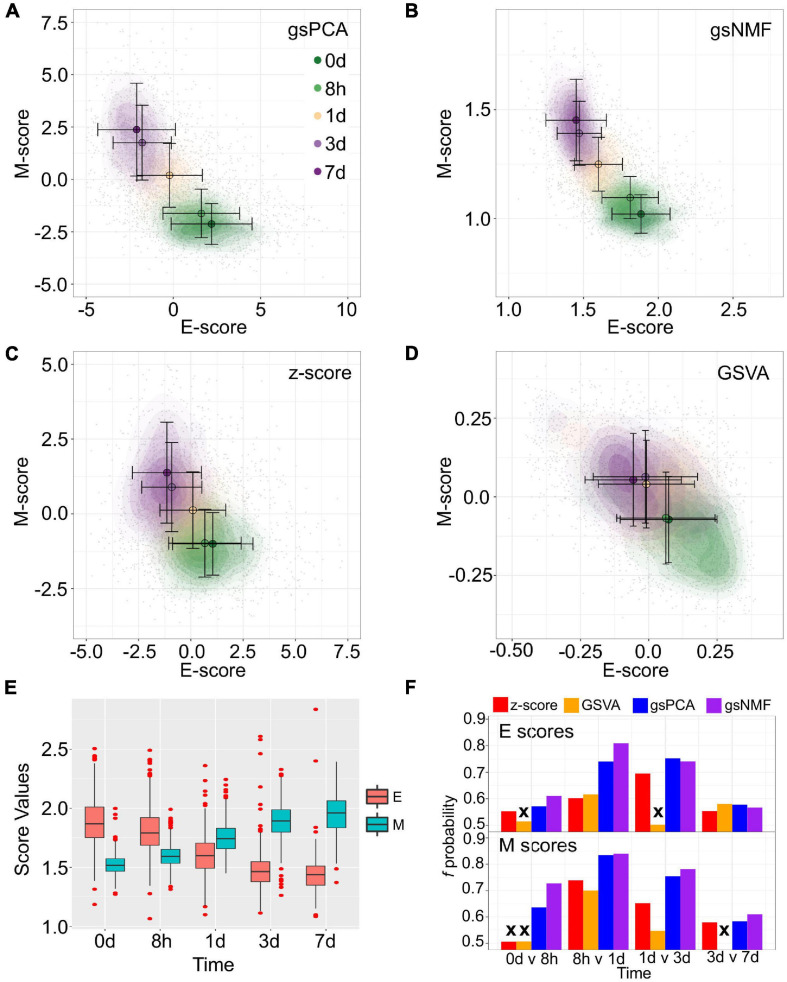
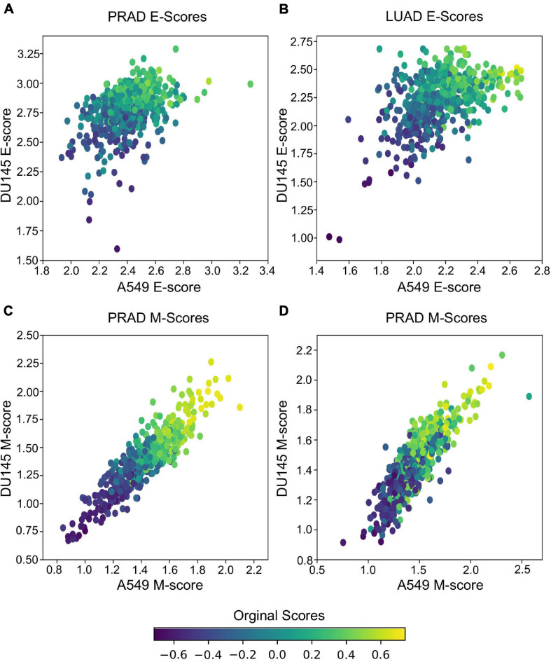
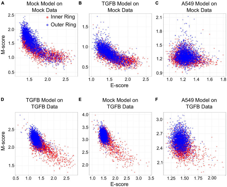
Large-scale transcriptome data, such as single-cell RNA-sequencing data, have provided unprecedented resources for studying biological processes at the systems level. Numerous dimensionality reduction methods have been developed to visualize and analyze these transcriptome data. In addition, several existing methods allow inference of functional variations among samples using gene sets with known biological functions. However, it remains challenging to analyze transcriptomes with reduced dimensions that are interpretable in terms of dimensions' directionalities, transferrable to new data, and directly expose the contribution or association of individual genes. In this study, we used gene set non-negative principal component analysis (gsPCA) and non-negative matrix factorization (gsNMF) to analyze large-scale transcriptome datasets. We found that these methods provide low-dimensional information about the progression of biological processes in a quantitative manner, and their performances are comparable to existing functional variation analysis methods in terms of distinguishing multiple cell states and samples from multiple conditions. Remarkably, upon training with a subset of data, these methods allow predictions of locations in the functional space using data from experimental conditions that are not exposed to the models. Specifically, our models predicted the extent of progression and reversion for cells in the epithelial-mesenchymal transition (EMT) continuum. These methods revealed conserved EMT program among multiple types of single cells and tumor samples. Finally, we demonstrate this approach is broadly applicable to data and gene sets beyond EMT and provide several recommendations on the choice between the two linear methods and the optimal algorithmic parameters. Our methods show that simple constrained matrix decomposition can produce to low-dimensional information in functionally interpretable and transferrable space, and can be widely useful for analyzing large-scale transcriptome data.

Keywords: EMT; RNA-sequencing data; dimensionality reduction; gene set analysis; single-cell ‘omics.

FIGURE 1

Schematic of the gene set non-negative matrix factorization (gsNMF)/gene set non-negative principal component analysis (gsPCA) analysis process. A diagram of the analysis process used in this study beginning with input data in the form of sequencing data and gene sets. gsNMF/gsPCA is applied to this data to generate a functional scoring or space in the form of component scores (see “Materials and Methods” section for details). These scores can be used in two ways. First, without further data labels, scores can be used to look at relationships between or across biological processes beginning with low-dimensional visualization to identify trends and putative groups. Quantities such as the correlation between different functional scores can be computed for analysis. In addition, the transferable nature of these models means that they can be used to infer the position of new data points and contributions of individual genes, which allows assessment of their importance. Screening can be done both between gene sets and within gene sets. Secondly, when data labels are present, different metrics can be used to assess the performance of a functional score in terms of capturing variance: the common language effect size or f-probability can be used to evaluate how well the functional score separates two distinct populations while the variance explained or R² can evaluate how much of the variation of a numeric variable representing biological progression, such as time, that the functional score can explain across the data.

FIGURE 2

Visualization of epithelial-mesenchymal transition (EMT) progression in TGF-β induced A549 cells by multiple scoring methods. (A–D) Contour plots of gene set scores of E (X-axis) and M (Y-axis) genes from four different scoring methods, gsPCA (A), gsNMF (B), z-score (C), and GSVA (D). Color indicates the time of TGF-β induction from 0 days (dark green) to 7 days (dark purple). Circles indicate the mean E- and M-score of samples from each time point and the associated error bars show the standard deviation. (E) A box-plot showing the distribution of E (red) and M (blue) scores across all five time points of TGF-β induction from the gsNMF model. Whiskers indicate the 1.5 inter-quartile range of each distribution while the red points indicate outliers beyond this range. (F) Bar chart of the f probability values for E (top) and M (bottom) scores between all consecutive pairs of time points. Color indicates the method used to produce the score: red is z-score, orange is GSVA, blue is gsPCA, and purple is gsNMF. Bars marked by an “x” indicates that the score did not significantly separate the samples from those time points (Mann–Whitney U-test, p < 0.05).

FIGURE 3

Predicting A549 samples from specific time points using gsNMF. (A) Scatter plot of E (X-axis) and M (Y-axis) scores for all TGF-β induction samples using gsNMF. Samples from different time points are indicated by color going from 0 days (dark green) to 7 days (dark purple). (B–D) Scatter plot of 0-day (green, B), 1-day (yellow, C), and 7-day samples (purple, D) inferred using a gsNMF model built with all other time points (gray). (E) A scatter plot of TGF-β induction samples with TGF-β reversion samples (i.e., 7 days induction followed by removal from TGF-β). Induction samples are labeled as in panel (A), while reversion samples are colored blue, with darker shade indicating longer time since removal. (F) Scatter plot of 3-day reversion samples (dark blue) inferred using a gsNMF model built with all non-reversion time points (gray).

FIGURE 4

Transferring gsNMF models between A549 and DU145 TGF-β induced samples. (A–D) Scatter plot of E (X-axis) and M (Y-axis) scores for different combinations of data and gsNMF model: (A) A549 model on A549 data, (B) DU145 model on A549 data, (C) A549 model on DU145 data, and (D) DU145 model on DU145 data. Samples from different time points are indicated by color going from 0 days (dark green) to 7 days (dark purple). (E,F) Comparison of E-scores of samples from A549 (E) and DU145 (F) data. The X-axis is the E-score from using the model from the same data set (A549 on A549 and DU145 by DU145), while the Y-axis is the E-score from the opposite model (DU145 on A549 and A549 on DU145). Samples from different time points are indicated by color going from 0 days (dark green) to 7 days (dark purple). (G,H) Comparison of M-scores of samples from A549 (G) and DU145 (H) data. The X-axis is the M-score from using the model from the same data set (A549 on A549 and DU145 by DU145), while the Y-axis is the M-score from the opposite model (DU145 on A549 and A549 on DU145). Samples from different time points are indicated by color going from 0 days (dark green) to 7 days (dark purple).

FIGURE 5

Transferring gsNMF models to TCGA data. (A,B) Scatter plots of E-scores for PRAD (A) and LUAD (B) from transferring gsNMF models built on A549 (X-axis) and DU145 (Y-axis) data. The color of individual points indicates the original GSVA based E-score of the TCGA data set. (C,D) Scatter plots of M-scores for PRAD (C) and LUAD (D) from transferring gsNMF models built on A549 (X-axis) and DU145 (Y-axis) data. The color of individual points indicates the original GSVA based M-score of the TCGA data set.

FIGURE 6

Transferring gsNMF models between temporal and spatial data sets. (A–C) Scatter plots of E (X-axis) and M (Y-axis) scores for Mock spatial data from gsNMF models built on different data sets: Mock spatial data (A), TGF-β induced spatial data (B), and TGF-β induced A549 temporal data (C). The color of the sample indicates whether it originates from a cell in the inner-ring (non-motile, red) or the outer ring (motile, blue). (D–F) Scatter plots of E (X-axis) and M (Y-axis) scores for TGF-β spatial data from gsNMF models built on different data sets: TGF-β induced spatial data (D), Mock spatial data (E), and TGF-β induced A549 temporal data (F). The color of the sample indicates whether it originates from a cell in the inner-ring (non-motile, red) or the outer ring (motile, blue).

FIGURE 7

Visualization of EMT progression in TGF-β induced A549 cells by multiple gene sets. (A–D) Contour plots of A549 functional space generated using gsNMF with different gene sets: E vs. M (A), KRAS knockdown up and down (B), non-malignant ovarian cancer up and down (C), and metastasis downregulation vs. angiogenesis downregulation (D). Color indicates the time of TGF-β induction from 0 days (dark green) to 7 days (dark purple). Circles indicate the mean gene set score of samples from each time point and the associated error bars show the standard deviation.

FIGURE 8

Visualization of trametinib treatment data by multiple gene sets. (A–D) Contour plots of trametinib treatment functional space generated using gsNMF with different gene sets: positive vs. negative gene regulation (A), KRAS overexpression up and down regulation (B), LEF overexpression up and down regulation (C), and positive cell-cycle regulation vs. drug response (D). Color indicates the time of trametinib treatment from 0 h (dark green) to 48 h (dark purple). Circles indicate the mean gene set score of samples from each time point and the associated error bars show the standard deviation.

References

1. Ashburner M., Ball C. A., Blake J. A., Botstein D., Butler H., Cherry J. M., et al. (2000). Gene ontology: tool for the unification of biology. The Gene Ontology Consortium. Nat. Genet. 25 25–29. - PMC - PubMed
1. Becht E., McInnes L., Healy J., Dutertre C.-A., Kwok I. W. H., Ng L. G., et al. (2019). Dimensionality reduction for visualizing single-cell data using UMAP. Nat. Biotechnol. 37 38–44. 10.1038/nbt.4314 - DOI - PubMed
1. Brunet J.-P., Tamayo P., Golub T. R., Mesirov J. P. (2004). Metagenes and molecular pattern discovery using matrix factorization. Proc. Natl. Acad. Sci. U.S.A. 101 4164–4169. 10.1073/pnas.0308531101 - DOI - PMC - PubMed
1. Chakraborty P., George J. T., Tripathi S., Levine H., Jolly M. K. (2020). Comparative study of transcriptomics-based scoring metrics for the epithelial-hybrid-mesenchymal spectrum. Front. Bioeng. Biotechnol. 8:220. - PMC - PubMed
1. Chen J., Zhang S. (2018). Discovery of two-level modular organization from matched genomic data via joint matrix tri-factorization. Nucleic Acids Res. 46 5967–5976. 10.1093/nar/gky440 - DOI - PMC - PubMed
LinkOut - more resources