Identifying indicator species in ecological habitats using Deep Optimal Feature Learning

Abstract

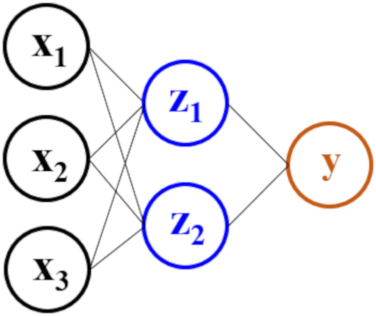
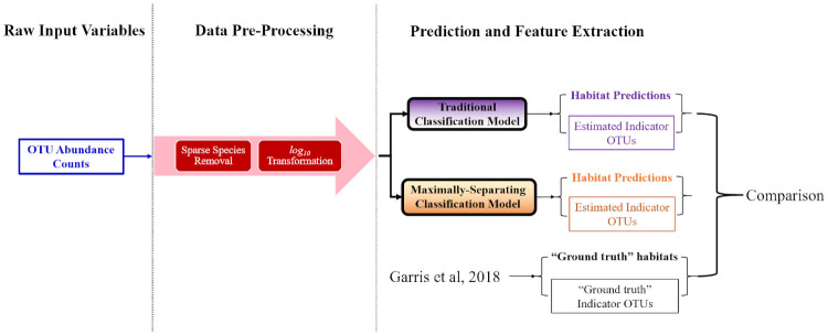
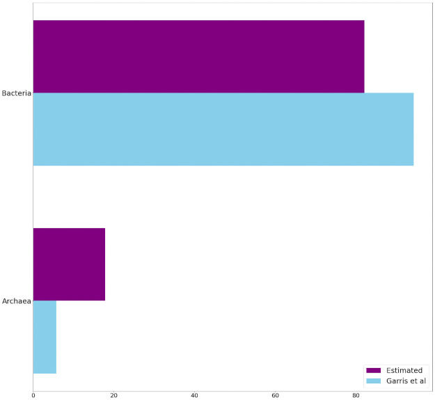
Much of the current research on supervised modelling is focused on maximizing outcome prediction accuracy. However, in engineering disciplines, an arguably more important goal is that of feature extraction, the identification of relevant features associated with the various outcomes. For instance, in microbial communities, the identification of keystone species can often lead to improved prediction of future behavioral shifts. This paper proposes a novel feature extractor based on Deep Learning, which is largely agnostic to underlying assumptions regarding the training data. Starting from a collection of microbial species abundance counts, the Deep Learning model first trains itself to classify the selected distinct habitats. It then identifies indicator species associated with the habitats. The results are then compared and contrasted with those obtained by traditional statistical techniques. The indicator species are similar when compared at top taxonomic levels such as Domain and Phylum, despite visible differences in lower levels such as Class and Order. More importantly, when our estimated indicators are used to predict final habitat labels using simpler models (such as Support Vector Machines and traditional Artificial Neural Networks), the prediction accuracy is improved. Overall, this study serves as a preliminary step that bridges modern, black-box Machine Learning models with traditional, domain expertise-rich techniques.

Fig 1. Overall data analysis workflow in block diagram form.

(Step 1): The collection of raw input data samples, as well as a corresponding set of labelled “ground-truth” targets. (Step 2): The pre-processing of raw input data into suitable structures for modelling, guided by any available domain or expertise knowledge. (Step 3): The training of several types of classification models (including Deep Learning), which maps inputs to their corresponding discrete class labels. (Step 4): The design of special objective function within a Deep Learning classification, which identifies a latent space with improved class separation. The most dominant latent features are then distinguished by the magnitude (ex. ℓ₂ norm) of the neural network weights.

Fig 2. Printout of pandas dataframes containing raw data collected directly from ecological sites.

(Left) Dataframe containing raw input variables. (Right) Dataframe containing output class labels.

Fig 3. Discovery of an optimally-separating latent feature space.

(Top Left) The high-dimensional and confounded raw inputs X makes class separation a challenging task.(Bottom Left) A case example including six microorganism species (A through F) which are entangled in the raw input space. (Top Right) A DL model which learns a latent space Z that optimally separates the classes. (Bottom Right) The disentanglement of the six species into distinct classes, which can be further aggregated into two major classes—Class 0 (A and B) and Class 1 (C through F).

Fig 4. Species abundance counts after each pre-processing transformation.

(Top) Distribution of counts from all 21721 species; the density is extremely skewed towards the low end. (Middle) Distribution of only the top 50 species by sum. (Bottom) Distribution of the top 50 species after a log₁₀ transformation. Rarer but higher-abundance species are now recognizable.

Fig 5. Histogram of maximum abundance counts.

Fig 6. Visualization of a linear separating hyperplane and separating margins in a 2-class SVM model.

Fig 7. Visualization of a classification problem with a non-linear separation boundary between the two classes.

(Left) The raw feature-space spanned by raw variables x₁ and x₂ renders linear separation impossible. (Right) A desired latent feature space which optimally separates the two classes. The goal of the DL model is to learn its coordinates, z₁ and z₂.

Fig 8. A two-layer neural network with a hinge-loss-like objective function.

Fig 9. Feature selection based on direction of optimal separation.

Fig 10. Selection of relevant input variables, by reverse-engineering matrix multiplication.

Fig 11. The overall data analysis workflow applied to the Mount Polley case study.

Fig 12. The ANN neuron architecture used in the Mount Polley case study.

Fig 13. The 4-layer ANN architecture used to classify the Fisher Iris dataset.

Fig 14. Visualization of data separation within the first ANN hidden layer.

(Left) Inter-class separation distance in the traditional ANN, between Class 2 (red) samples and Class 1 (black) samples. (Right) Inter-class separation distance in the optimally-separating ANN.

Fig 15. Inter-class separations in the traditional ANN.

Black samples belong to the undisturbed class. Red samples belong to the disturbed class. Only the first 4 out of the total 5000 runs are shown.

Fig 16. Inter-class separations in the optimally-separating ANN.

The separations are noticeably larger than those in Fig 15. Black samples belong to the undisturbed class. Red samples belong to the disturbed class. Only the first 4 out of the total 5000 runs are shown.

Fig 17. Taxonomic comparison of indicator species at the domain level.

Blue bars represent the indicators identified by Garris et al [34]. Purple bars represent the indicators identified by our proposed feature extractor. The horizontal axis represents the percentage of indicators belonging to each species.

Fig 18. Taxonomic comparison of indicator species at the phylum level.

Blue bars represent the indicators identified by Garris et al [34]. Purple bars represent the indicators identified by our proposed feature extractor. The horizontal axis represents the percentage of indicators belonging to each species.

Fig 19. Taxonomic comparison of indicator species at the class level.

Blue bars represent the indicators identified by Garris et al [34]. Purple bars represent the indicators identified by our proposed feature extractor. The horizontal axis represents the percentage of indicators belonging to each species.

References

-
- Rajput DS, Basha SM, Xin Q, Gadekallu TR, Kaluri R, Lakshmanna K, et al.. Providing diagnosis on diabetes using cloud computing environment to the people living in rural areas of India. Journal of Ambient Intelligence and Humanized Computing. 2021; p. 1–12.
- Podani J, Csányi B. Detecting indicator species: Some extensions of the IndVal measure. Ecological Indicators. 2010;10(6):1119–1124. doi: 10.1016/j.ecolind.2010.03.010 - DOI
- Penczak T. Fish assemblage compositions after implementation of the IndVal method on the Narew River system. Ecological modelling. 2009;220(3):419–423. doi: 10.1016/j.ecolmodel.2008.11.005 - DOI
MeSH terms
LinkOut - more resources
Full Text Sources