. 2021 Sep 21;118(38):e2109729118.
doi: 10.1073/pnas.2109729118.

Geometry of gene regulatory dynamics

Affiliations

Geometry of gene regulatory dynamics

David A Rand et al. Proc Natl Acad Sci U S A. .

Abstract

Embryonic development leads to the reproducible and ordered appearance of complexity from egg to adult. The successive differentiation of different cell types that elaborate this complexity results from the activity of gene networks and was likened by Waddington to a flow through a landscape in which valleys represent alternative fates. Geometric methods allow the formal representation of such landscapes and codify the types of behaviors that result from systems of differential equations. Results from Smale and coworkers imply that systems encompassing gene network models can be represented as potential gradients with a Riemann metric, justifying the Waddington metaphor. Here, we extend this representation to include parameter dependence and enumerate all three-way cellular decisions realizable by tuning at most two parameters, which can be generalized to include spatial coordinates in a tissue. All diagrams of cell states vs. model parameters are thereby enumerated. We unify a number of standard models for spatial pattern formation by expressing them in potential form (i.e., as topographic elevation). Turing systems appear nonpotential, yet in suitable variables the dynamics are low dimensional and potential. A time-independent embedding recovers the original variables. Lateral inhibition is described by a saddle point with many unstable directions. A model for the patterning of the Drosophila eye appears as relaxation in a bistable potential. Geometric reasoning provides intuitive dynamic models for development that are well adapted to fit time-lapse data.

Keywords: Morse–Smale; Turing model; Waddington landscape; bifurcation; gene network.


Conflict of interest statement

The authors declare no competing interest.

Figures

Fig. 1.
Fig. 1.
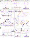
Representations of MS systems. (A) The symbol set used consistently to describe elements of the phase space or parameter space. (B) An MS system with three attractors and two saddles showing the stable (red) and unstable (blue) manifolds of the saddles. Contours of a potential are shown in gray. In this system, the unstable manifolds meet at the attractor B in a cusp-like shape. (C) In this MS system, which also has three attractors, the unstable manifolds of the saddles make up a smooth curve. (D, Upper) Two examples of DAGs corresponding to the system in B, left side and the CEU of Fig. 5D (B, right side). (D, Lower) The decision structures associated with the DAGs above them. The filled circles represent the attractors, and a connection between attractor A and B means that a cell whose state sits at A (B) can transition to B (A) via a saddle-node bifurcation that destroys A (B). Thus, the connections characterize the escape routes and possible decisions. The connections also correspond to the index 1 saddles in the system that connect A and B. Some escape routes wrap around an index 2 saddle as shown and indicated by a triangle. To minimize the numbers of decision diagrams, we do not distinguish cases where multiple saddles connect the same two fixed points (SI Appendix, section I.7). (E and F) The two simplest bifurcations: the local saddle node and the global heteroclinic flip. These are the main events underlying decision making in our dynamical systems. (E) A saddle-node or fold bifurcation. As θ increases through zero, a saddle and an attractor are born, which then separate with a distance of order θ. (F) The configuration shown in A can flip to one where the saddle a is connected to C instead of B via a heteroclinic flip. To do this, it passes through the intermediate state shown where there is a heteroclinic connection in which the unstable manifold of the saddle a connects to the saddle at b. (G) An example of a compact landscape involving a repellor. We have taken a case where the attractor is close to the saddle to illustrate that the attractor can move around the circular unstable manifold and collide, undergoing a saddle-node bifurcation and turning the unstable manifold into a limit cycle. This is called an SNIC (Saddle Node on Invariant Cycle) bifurcation. Although it is important to be aware of such bifurcations, we do not consider them anymore since the existence of a limit cycle moves us out of the gradient-like rest point–only systems.
Fig. 2.
Fig. 2.
The hierarchy of elementary catastrophes obtained by coupling two bistable systems. These describe all generic local bifurcations of potentials depending on r4 parameters. If hθ is such a generic family, then there are coordinates (x1,,xn) on phase space such that hθ=fθ(y)+ρ+1nϵixi2 where fθ(y) represents one of the elementary catastrophes in the figure, ρ=1or2, and the remaining phase space variables can be reduced to a diagonal quadratic form where ϵi=±1. Several of these polynomials are prototypes for the parameterized landscapes. A precise statement is in ref. .
Fig. 3.
Fig. 3.
Building complexity from bistable landscapes using one- and two-dimensional perturbations. The legend is as shown and follows the key in Fig. 1A. (A) We distinguish between these two three-attractor systems, even though they are topologically conjugate, because in applications, the allowed transitions are different. The red attractor cannot undergo a saddle-node bifurcation when the unstable manifolds of the saddles merge in a cusp. The attractors represent biological states that are not equivalent, as they would be under topological conjugacy. (Upper) All the rest points lie on a smooth curve defined by the unstable manifolds of the saddles. (Lower) The unstable manifolds of the saddles meet at a central sink in a cusp with a common tangency. (B) Fold bifurcations add an extra saddle–sink pair to the bistable system. The new attractor is marked in blue. (C–H) The allowed bifurcation sets for three and fewer fixed points when two parameters are varied. The colored curves denote fold bifurcations where the like-colored attractor disappears. (C) Dual cusp. The new attractor in blue, and the saddle is inserted in the middle. For this to occur, the fold bifurcation curve must contain at least one cusp point. (D) Standard cusp. A bistable system has a third attractor added. The cusps in C and D are defined by the discriminant of the same third-order polynomial representing either a source and two saddles or a saddle and two attractors (cf Fig. 2). (E and F) Crossing points. Two fold bifurcation curves can intersect transversally, creating a region with a single attractor and a region where there are three attractors. (E) One of the two bifurcation curves involves the central attractor, and then, the attractors must lie on a smooth curve. (F) In this case, the curves correspond to peripheral attractors, and then, both smooth and cusped unstable manifolds are possible. (G and H) There can be a (codimension-2) point on the fold bifurcation curve where the unstable manifold of the top saddle undergoes a heteroclinic flip as shown. Generically, these heteroclinic flips occur on a curve (green). (G) When the source saddle bifurcates away, the flip curve in green intersects the fold bifurcation curve transversely. (H) When the target saddle is destroyed in a fold bifurcation, the flip curve generically terminates in a cusp (SI Appendix).
Fig. 4.
Fig. 4.
The legend is the same as in Figs. 1A and 3. (A) Over part of the boundary P of a two-dimensional domain of parameter space P, we assume we have an S-shaped bistable section and that the system is monostable over the rest of P. Then, it follows that under very mild conditions (SI Appendix, section I.4E) inside P, there must be at least one cusp (ref. has n=1 case). This is because there must be a fold curve joining the two folds shown, and on this fold curve, the two folds shown have opposite orientations. (B–G) Local rules governing the disposition of cusps and crossings in the boundary of a three-attractor MS component. X is always the central attractor, P, P peripheral. (B) The orientation of the fold bifurcation involving the central attractor determines the possible transverse crossings of the fold bifurcation curve. On the black fold bifurcation curve, the central attractor bifurcates with the saddle to its right (connected to red); thus, the only allowed crossing is the bifurcation of the yellow attractor with its saddle. (C) The peripheral attractor involved in the fold constrains the possible crossings of the fold bifurcation curve. (D) Standard cusp. Fold bifurcation curves crossing the cusp’s branches satisfy the conditions in B and C. (E) Dual cusp. Fold bifurcation curves crossing the cusp’s branches satisfy the conditions in B and C, and the crossings imply the existence of the cusp. (F) The opposite orientations of the folds of the central attractor on the two fold bifurcation curves as shown imply the existence of a cusp. (G) If QQ is a single-fold bifurcation curve, certain consecutive crossings are not possible. By B, Q=P, but P cannot intersect itself; so, if Q=X, then the next intersection can only be with P via D.
Fig. 5.
Fig. 5.
Minimal three-attractor MS components (light blue). The legend is the same as in Figs. 1A or 3. The color of a fold bifurcation curve indicates the attractor that bifurcates on it. (A) The minimal MS components containing a dual cusp. Inset shows the minimal system involving a dual and standard cusp. The MS components with less than or equal to two attractors are a subset of this for the dual-cusp case. (B) Minimal MS component for a standard cusp. Inset in the pink box shows a simple alternative configuration replacing the red curve at the bottom of the cusp. (C) The same for a standard cusp and a flip curve. Note that for parameters near a cusp point, the connector among the three attractors will be smooth. The intersection of the flip curve (green) is cusped when it hits the fold for the central attractor and transverse when the peripheral (red) attractor disappears. There is a second curve emanating from the cusp in the flip curve where the connector changes from smooth to cusped. (D) The CEU. Inside the MS component boundary and outside the triangular hypocycloid BC, there are three attractors and two saddles. This dynamical system can be obtained by taking the gradient dynamical system of the potential associated with the potential fθ(x,y)=x4+y4+x32xy2+a(x2+y2)+θ1x+θ2y, with respect to a generic Riemannian metric. The term x4+y4 is added to the usual polynomial for Thom’s elliptic umbilic in order to make the dynamical system compact. It has the effect of adding the three attractors and the outer fold bifurcation curves to the three saddles. The sign of the parameter a controls whether the central rest point is an attractor or repellor. By the MS inequalities (6), this is a minimal effect.
Fig. 6.
Fig. 6.
A symmetric three-cell or gene network with mutual repulsion and the elliptic umbillic conformation (Fig. 5D). The outer colored lines are the fold curves when one of the states disappears (three attractors become two). At the points A, B, and C, there is one stable rest point and four with eigenvalues (1,0,1) (i.e., the intersection of two fold lines). The inner black contour consists of three fold lines, and inside, it is an index 2 saddle, three index 1 saddles, and three attractors.
Fig. 7.
Fig. 7.
A potential constructed for a prototype activator–inhibitor system with flows shown in green. Contours of the potential, which is defined as the integral of the vector field along the trajectory to the stable fixed point, are shown going from low (blue) to high (red) potential. The red arrows on one of the contour lines show the flow from the gradient of the potential. Since the equations have a nonzero curl, a metric is required to align the red and green arrows. The construction does not work near the fixed points, but a separate potential and metric can be defined there (18) and glued to the global potential (details are in SI Appendix, section II.2). (Insets) Plots of the contour lines in red and flow magnified near the upper fixed point and the saddle are also shown.
Fig. 8.
Fig. 8.
Behavior of Eq. 2. (A) Values of inhibition h for which the ȧ equation has saddle-node bifurcations. When h from neighboring cells is <0.37, only the a=1 state is stable, bistability persists for 0.37<h<0.63, and only the a=0 state exists for larger h. The diagonal is shown in black. (B) Eight cells on the circle with a kernel chosen to allow only two cells with a=1 at the end. The time to reach steady state can vary by 2× depending on whether a third cell hangs close to the saddle point as seen here vs. Fig. 9.
Fig. 9.
Fig. 9.
Two potential models for Eq. 2 run with the same initial conditions. (A) The potential in Eq. 3 with the inverse metric extending to the origin. (B) The inverse metric near the origin now matches Eq. 2.
Fig. 10.
Fig. 10.
A sector of the tangent plane to the unstable manifold at the saddle for a discrete version of Eq. 4 with N=7 cells. The blue arrows show the trajectories of the potential fit with different initial conditions chosen at equally spaced angles. The red arrows show the projection of the actual equations on the tangent plane. Arrows are plotted at equal times and so, give the approximate velocity.
Fig. 11.
Fig. 11.
The continuous Turing PDE (Partial Differential Equation) is solved and projected onto the variables z1 and z2 in Eq. 6 by simply doing a linear projection onto the Fourier modes (zi=rieiθi). (A) The streamlines of Eq. 6 in the space of the two radii with the angles set to zero showing a two-dimensional projection of the four-dimensional unstable manifold. The callouts show the terminal profiles of a(x) at the saddle with two peaks and the fixed point with one. The initial condition is a(x)=0.01cos(2x)+0.001cos(x). (B) Eq. 6 implies that the angles stably lock together with 2θ1θ2=0. This is shown with blue dots for the actual Turing model and red for the potential fit for various initial conditions. (C) A saturation function is required to match the solution in the tangent space in (a,h) to a(x) in physical space x. The solution of the continuous system (blue) is compared with a sigmoidal saturation of the tangent space flow (red) for the red cross-over trajectory in A.
Fig. 12.
Fig. 12.
(A) A model in two spatial dimensions leads to the formation of three blobs, each of which are slightly different because of randomness in the parameters and initial conditions. The blobs are shown at two different time points, demonstrating that the left and right ends form at different times. Since the blobs have spherical symmetry, the profile is first averaged over angles and then projected onto the Bessel function J0(R) being the first term in a Fourier–Bessel series, where R is a scaled radial coordinate in space. (B) The simulated two-dimensional dynamics are projected onto the tangent plane (dots) for the left (red) and right (blue) blobs in A. The data are fit very well by the radial part of Eq. 5 (curve) with parameters specific to each blob. The space–time profiles in A are then fit by a sigmoid depending on r(t) from Eq. 5 and J0(R) (SI Appendix, section II.4).
Fig. 13.
Fig. 13.
Dynamics for the one-dimensional morphogenic furrow from Eq. 8 for n = 30, where every fourth cell is active. The wave appears to slow toward the end since the long-range activator b is diffusing out the right-hand boundary. For the same reason, the plateau in ai is a bit lower at the end. Solutions with periods 2 to 5 all have energies below the initial state, but only period 4 appears behind the wave.

References

    1. Smale S., On gradient dynamical systems. Ann. Math. 74, 199–206 (1961).
    1. Meyer K. R., Energy functions for Morse-Smale systems. Am. J. Math. 90, 1031–1040 (1968).
    1. Smale S., Differentiable dynamical systems. Bull. Am. Math. Soc. 73, 747–817 (1967).
    1. Guckenheimer J., Holmes P., Nonlinear Oscillations, Dynamical Systems, and Bifurcations of Vector Fields (Springer Science & Business Media, 2013), vol. 42.
    1. Newhouse S., Peixoto M., There is a simple arc joining any two Morse-Smale flows. Asterisque 31, 15–41 (1976).

Publication types

LinkOut - more resources