Compound climate extremes driving recent sub-continental tree mortality in northern Australia have no precedent in recent centuries

Abstract

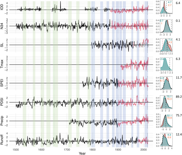
Compound climate extremes (CCEs) can have significant and persistent environmental impacts on ecosystems. However, knowledge of the occurrence of CCEs beyond the past ~ 50 years, and hence their ecological impacts, is limited. Here, we place the widespread 2015-16 mangrove dieback and the more recent 2020 inland native forest dieback events in northern Australia into a longer historical context using locally relevant palaeoclimate records. Over recent centuries, multiple occurrences of analogous antecedent and coincident climate conditions associated with the mangrove dieback event were identified in this compilation. However, rising sea level-a key antecedent condition-over the three decades prior to the mangrove dieback is unprecedented in the past 220 years. Similarly, dieback in inland forests and savannas was associated with a multi-decadal wetting trend followed by the longest and most intense drought conditions of the past 250 years, coupled with rising temperatures. While many ecological communities may have experienced CCEs in past centuries, the addition of new environmental stressors associated with varying aspects of global change may exceed their thresholds of resilience. Palaeoclimate compilations provide the much-needed longer term context to better assess frequency and changes in some types of CCEs and their environmental impacts.

Figure 1

(a) Average sea level anomalies March 2013–February 2015; (b) Average sea level anomalies, September 2015–February 2016. Base period for these anomalies is 1993–2012 (see https://www.aviso.altimetry.fr/en/data/products/sea-surface-height-products/global/gridded-sea-level-anomalies-mean-and-climatology.html); (c) SST anomalies Sep 2015–Mar 2016. (d) Sea level data from Freemantle and Darwin showing very close relationship between the two; (e) Location of land-based palaeo-proxy records used in this study and climate model indices as well as the Niño 3.4 box and the east and west poles of the IOD index. Figure created using QGIS 3.10.

Figure 2

Left panel: Time series (z-scores relative to the 1961–90 period) of reconstructed and instrumental indices (IOD, Niño3.4) and climate variables (Sea level, maximum temperature; SPEI3, PDSI, precipitation (AWAP data); Alligator River run off) relevant for northern Australia. For sea level, red line is the non-detrended sea level data while grey line is the detrended data. Right panel: associated probability distributions, red is for reconstructed series, and teal for instrumental data. Vertical black lines show where in the distribution the 2015–16 value fell. Red line in sea level distribution shows value for 2015–16 once data detrended, black line is for non-detrended data. Numbers in upper left or right relate to the empirical probability (as percentages) of experiencing an event in that variable at least as extreme as that in 2015. Colours match the respective distributions. For sea level, figures are based on detrended sea level data.

Figure 3

(a) Comparison of reconstructed parameters and instrumental data. Reconstructions are red and instrumental data in teal. Statistics next to each plot have been drawn from the original publications (Table 1). Those for the runoff reconstruction have been averaged across the early and late, and (for R²c), the whole calibration periods. Note that the runoff reconstruction based on proxies as described in Verdon-Kidd et al. (2017) extends only to 1975 after which it is based solely on streamflow simulated from rainfall, hence the almost perfect fit from 1976 to 2011. (b) The number of hydroclimate reconstructions that record single year events. Also shown are those years for which each of the IOD, Nino 3.4 and sea level data shows an event. Background shading indicates number of hydroclimate proxies available for each year.

Figure 4

Hydroclimate and native tree deaths. (a) Monthly mSPEI3 values for the monsoonal north (for the box—17.75S 128.25E–10.25S–142.75E) from 1950 to 2020 (data source: https://spei.csic.es/database.html). Black dotted lines show the period from January 2015 to December 2016. Lowest mSPEI3 value recorded in June 2016. Red dotted line shows start of 2019. (b) Number of months per decade for which mSPEI3 < 0 (yellow), mSPEI3 < − 0.5 (coral), mSPEI3 < − 1 (dark red). (c) Distribution of 6-year non-overlapping averages of the March–May SPEI3 (reconstruction + instrumental). Dashed line shows the average SPEI3 value for the 2014–2019 period. (d) Runs of wet and dry years consistent with criteria described in main text according to the four different hydroclimate indices. A run of dry years is defined as at least 4 of 5 consecutive years with a value of − 0.5 s below the mean for the 1961–90 reference period. Longer dry periods may include up to two non-event years. Wet events include at least 10 wet years (+ 0.5 s) over a period of no more than 12 years. Y-axis indicates number of years events persisted. Negative values indicate extended dry events, positive values reflect extended wet events according to the criteria applied (Methods).

References

1. IPCC Managing the risks of extreme events and disasters to advance climate change adaptation. In A Special Report of Working Groups I and II of the Intergovernmental Panel on Climate Change (eds Field, C. B. et al.) 582 (Cambridge University Press, 2012).
1. Zscheischler J, et al. Future climate risk from compound events. Nat. Clim. Change. 2018;8:469–477. doi: 10.1038/s41558-018-0156-3. - DOI
1. Zscheischler J, et al. A typology of compound weather and climate events. Nat. Rev. Earth Environ. 2020;1(7):1–15. doi: 10.1038/s43017-020-0060-z. - DOI
1. Wahl T, Jain S, Bender J, Meyers SD, Luther ME. Increasing risk of compound flooding from storm surge and rainfall for major US cities. Nat. Clim. Change. 2015;5:1093–1097. doi: 10.1038/nclimate2736. - DOI
1. Bevacqua E, et al. More meteorological events that drive compound coastal flooding are projected under climate change. Commun. Earth Environ. 2020;1:47. doi: 10.1038/s43247-020-00044-z. - DOI - PMC - PubMed
Publication types