Artificial Intelligence Applied to Battery Research: Hype or Reality?

Abstract

This is a critical review of artificial intelligence/machine learning (AI/ML) methods applied to battery research. It aims at providing a comprehensive, authoritative, and critical, yet easily understandable, review of general interest to the battery community. It addresses the concepts, approaches, tools, outcomes, and challenges of using AI/ML as an accelerator for the design and optimization of the next generation of batteries─a current hot topic. It intends to create both accessibility of these tools to the chemistry and electrochemical energy sciences communities and completeness in terms of the different battery R&D aspects covered.

Figure 1

Overall working principles of a ML approach for supervised/unsupervised and classification/regression methods. For simplicity, here classification is represented as the only application of unsupervised ML, despite other applications, for instance dimensionality reduction, existing.

Figure 2

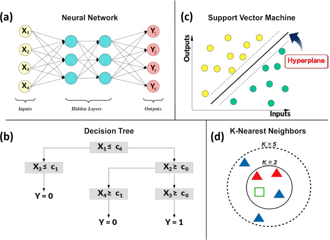
Workflows of some of the most common ML techniques: (a) neural network; (b) decision tree; (c) support vector machine; (d) k-nearest neighbors (k-NN).

Figure 3

Example of GP regression. The standard deviation refers to the error associated with the predictions.

Figure 4

Deep learning architectures for generative modeling.

Figure 5

Inverse design with deep learning models.

Figure 6

Percentage of reviewed articles applying AI or ML to the different battery-related topics discussed in this Review. This analysis was performed on ∼200 scientific articles.

Figure 7

Infographic on the ML methods recently used in the literature to search for new battery materials with specific target properties, including the corresponding nature (calculated vs experimental data) of the employed databases.

Figure 8

Eight different material descriptors to represent a 9,10-antraquinone-2,7-disulfonic acid (AQDS) molecule used in organic redox flow batteries. Figure reproduced with permission from ref (126). Copyright 2018 American Association for the Advancement of Science.

Figure 9

Schematic representation of the procedure followed by Min et al. to establish optimal synthesis parameters for Ni-rich NMC cathode materials. Figure adapted with permission from ref (156). Copyright 2018 Springer.

Figure 10

Schematic representation of the working procedure followed by Joshi et al. and some examples of results. Figure adapted with permission from ref (159). Copyright 2019 American Chemical Society.

Figure 11

Schematic workflow of a BO-based model to search for DFT-computed Li- and Na-ion migration energies (E_b) in tavorite AMXO₄Z compounds. Figure reproduced with permission from ref (164). Copyright 2018 Springer.

Figure 12

Preliminary results of an ANN trained on HCE LiTFSI in ACN by Johansson’s and MIT groups.^,,

Figure 13

Complexity of a typical battery solid electrolyte interphase (SEI) increases continuously, from the molecular level to the macroscale. Assessing the state of the interphase requires therefore the combination of a range of simulation (blue), electrochemical (orange), and characterization (green) approaches. Figure reproduced with permission from ref (129). Copyright 2019 Elsevier.

Figure 14

Schematic workflow of an ANN-potential-assisted genetic algorithm used to construct the phase diagram of amorphous Li_xSi. Figure reproduced with permission from ref (187). Copyright 2018 AIP publishing.

Figure 15

(A) Recursive partitioning analysis of the effect of synthetic parameters (elemental compositions, annealing, and deposition temperatures) on the percentage of Li_3xLa_2/3–xTiO₃ observed within the samples deposited. (B) NN-based predicted total ionic conductivities in Li_3xLa_2/3–xTiO₃ as a function of composition using empirical results as a training data set. Figure reproduced with permission from ref (200). Copyright 2011 American Chemical Society.

Figure 16

Infographic on the ML methods recently used in the literature to optimize and/or better understand manufacturing processes, including the corresponding nature (simulated vs experimental data) of the employed databases.

Figure 17

Schematic of typical LIB electrode and cell manufacturing processes. Reprinted with permission from “The Future of Battery Production for Electric Vehicles”. Copyright 2018 The Boston Consulting Group Inc. All rights reserved.

Figure 18

Electrode capacity at 15C vs formulation for (top) 0 wt %, (middle) 10 wt %, and (bottom) 20 wt % of carbon black (C65). LiFePO₄ (LFP) formulations are reported on the first and second columns, while Li₄Ti₅O₁₂ (LTO) formulations are reported on the third and fourth ones. Polyvinylidene fluoride (PVdF) is used as a binder in the first and third columns, while polyethylene-co-ethyl acrylate-co-maleic anhydride (TPE), in the second and fourth ones. The lines are iso-capacities with values given in mAhg^–1, where the electrode weight without the current collector is used to normalize the capacity. The empty areas are out of the study boundaries. Figure reproduced with permission from ref (77). Copyright 2020 American Chemical Society.

Figure 19

Schematic of a LIB manufacturing process chain utilizing a data-driven approach. Figure reproduced with permission from ref (107). Copyright 2020 Wiley.

Figure 20

Concept of a LIB factory data warehouse and its connection to data mining. Figure reproduced with permission from ref (107). Copyright 2020 Wiley.

Figure 21

SVM classification in terms of the dried electrode mass loading levels (low, medium, or high) as a function of the slurry viscosity and S-to-L ratio for different AM amounts: (A) 92.7%, (B) 94%, (C) 95%, and (D) 96%. Figure reproduced/adapted with permission from ref (220). Copyright 2020 Wiley.

Figure 22

SVM classification in terms of the dried electrode porosity (low, medium, or high) as a function of the slurry viscosity and S-to-L ratio for different AM (NMC) weight contents: (A) 92.7%, (B) 94%, (C) 95%, and (D) 96%. Panels A′ and D′ provide the interpretation on the lack of low porous electrodes in panel A and their existence in panel D, respectively. Figure reproduced/adapted with permission from ref (220). Copyright 2020 Wiley.

Figure 23

Multicriterial analysis of influencing factors on three FPPs studied by Thiede et al. Figure reproduced with permission from ref (223). Copyright 2019 Elsevier.

Figure 24

Overall workflow of the hybrid methodology presented in ref (21). Experimental and/or physics-based modeling results capturing the impact of manufacturing parameters on electrode mesostructure properties (A) are embedded in a D-DEMG algorithm (B) that generates electrode mesostructure associated to specific manufacturing conditions. These mesostructures are analyzed, building the data set (C) that is used to train and validate ML algorithms. This allows describing mathematically the correlations between electrode properties and process variables as manufacturing conditions (D). Dark gray arrows represent the steps considered along the case study presented in ref (21), while light gray ones indicate future perspectives of this methodology. Figure reproduced with permission from ref (21). Copyright 2020 Elsevier.

Figure 25

(A) Example of outputs (for the case of the electrolyte tortuosity) from Duquesnoy et al.ε_init stands for the electrode porosity prior the calendaring, the color scale indicates the AM wt %, and the values reported in the graph indicate the electrode porosity after the calendering for certain calendering pressure. (B) Correlations between calender pressure and electrode properties before calendering and several mesoscale properties studied by Duquesnoy et al. Green and red colors represent direct and inverse relations, respectively, while the size of the circles indicates the degree of correlation (i.e., big circles, strong correlation) obtained by a PCA-based study. The last column indicates the sense to which the property should be tuned (i.e., maximize or minimize the property) in order to increase the energy density. Figure adapted with permission from ref (21). Copyright 2020 Elsevier.

Figure 26

(A) Schematic of the particle swarm optimization algorithm developed by Lombardo et al. Left, initial guesses of the PSO algorithm in terms of FF parameter values for the CGMD simulations (linked to their associated 3D slurry structures). Right, the PSO algorithm converged to the FF parameter values needed to match the targeted experimental results. For each set of FF parameter values, a schematic of the associated slurry 3D structure is reported as well. In Lombardo et al., eight CGMD simulations were launched in parallel for each iteration. (B) PSO merged with a DNN algorithm to speed up the algorithm convergence. For each iteration, dots represent FF parameter values tested by the PSO, while the star indicates the ones predicted by the DNN. All the results of each iteration were added to the data set in order to improve the DNN accuracy. At the end right, a comparison of experimental (line) and simulated (dots) results is reported. Figure adapted with permission from ref (230). Copyright 2020 Wiley.

Figure 27

Infographic on the ML methods recently applied to materials and electrode characterization, including the corresponding nature (calculated vs experimental data) of the employed databases.

Figure 28

Performance of five ML classifiers (kNN, RF, CNN, MLP, and SVC) on coordination environment classification. (A) Accuracy and (B) Jaccard score for the five ML classifiers broken down by elemental categories, namely, alkali metals, alkaline earth metals, transition metals (TMs), post-transition metals, metalloids, and carbon. (C) Relationship between the RF model’s classification accuracy and the data set size. (D) Relationship between the RF model’s classification accuracy and the training label entropy. Cation elements with a classification accuracy less than 0.85 are labeled in parts C and D. Figure reproduced with permission from ref (245). Copyright 2020 Elsevier.

Figure 29

(a) NN data architecture and workflow for crystal space group determination from experimental high-resolution atomic images and diffraction profiles. Seeding the prediction of crystallography is a hierarchical classification using a one-dimensional CNN model. (b) XRD data preparation protocol. Comparison between experimental and simulated XRD patterns for Al₂O₃, Li₂O, SrO, and SrAl₂O₄. Green and brown lines stand for experimental and simulated XRD patterns, respectively. (c) A scheme of the automated determination of crystal symmetry based on diffraction experiments. (d) The ratio of correctly classified structures versus space-group number from the CNN model. Marker size reflects the relative frequency of the space group in the training set. (e) This CNN model trained by the data augmentation technique would not only open numerous potential applications for identifying XRD patterns for different materials. (a) Figure adapted with permission from ref (248). Copyright 2019 American Association for the Advancement of Science. (b) Figure reproduced with permission from ref (249). Copyright 2020 Springer. (c) Figure reproduced with permission from ref (250). Copyright 2020 Springer. (d) Figure reproduced with permission from ref (251). Copyright 2019 International Union of Crystallography. (e) Figure reproduced with permission from ref (252). Copyright 2020 American Chemical Society.

Figure 30

(a) The workflow of the GAN reconstruction (GANrec) algorithm. The input is a tomography sonogram (X-ray ptychographic tomography data), which is transformed into a candidate reconstruction by the GAN generator. The candidate reconstruction is projected to a model sinogram by a Radon transformation. The model sinogram is compared with the input sinogram by the discriminator of the GAN, in which a GAN loss is obtained based on this comparison. The weights of the generator and discriminator of the GAN evolved by optimizing the GAN loss. (b) The missing-wedge problem in electron tomography is solved using GAN. (c) Two different reconstructions of a noisy simulated data set, on the left, the results of conventional reconstruction with a high level of noise and, on the right, the same image after de-noising with TomoGAN. (a) Figure reproduced with permission from ref (266). Copyright 2020 International Union of Crystallography. (b) Figure reproduced with permission from ref (267). Copyright 2019 Springer. (c) Figure reproduced with permission from ref (268). Copyright 2020 The Optical Society.

Figure 31

(a) Subsurface porosity map measured through the depth of the sample for the pristine and the failed electrolyte pellet. (b) Cross section through the EBSD image of NMC depicting grain boundaries using FIB-EBSD. Segmentation result of the watershed algorithm in which each region is colored individually after removing regions outside of the considered NMC particle. (c) A depth-dependent particle fracturing profile in the Ni-rich NMC electrode revealed by X-ray computed tomography. The scale bar is 20 μm. (d) The 3D image of the segmentation results over two regions of interest, with the carbon binder domain (CBD) set to be transparent for a better visualization of the NMC particle (orange) and the pores (gray–blue). (e) Results on the graphite electrode with a map of Bayesian CNN uncertainty, which is focused around the light gray edges of the material in the original slice, while the Monte Carlo dropout network uncertainty is pixelated. (a) Figure adapted with permission from ref (271). Copyright 2020 American Chemical Society. (b) Figure adapted with permission from ref (272). Copyright 2021 Elsevier. (c, d) Figure reproduced/adapted with permission from ref (273). Copyright 2020 Springer. (e) Figure reproduced with the authors’ permission from ref (274).

Figure 32

(A) Workflow of the GAN-based model proposed by Gayon-Lombardo et al. able to learn and reproduce 3D electrode microstructures. (B) Workflow of the GAN-based model developed by Kench et al., unlocking the use of 2D images to build 3D electrode microstructures. (A) Figure reproduced with permission from ref (121). Copyright 2020 Springer. (B) Figure reproduced with permission from ref (122). Copyright 2021 Springer.

Figure 33

(a) The four misclassified examples of micrographs with defects by the VGG19 fine-tuned model. (b) Overview of the model development. The following three classes of particle pairs are differentiated: BROKEN: The particle pair belonged to the same particle before it broke apart during the thermal runaway. WATERSHEDSEP: The particle pair corresponds to two touching particles in the tomographic image, which are split by the watershed transformation. PARTICLESEP: The particle pair consists of unrelated, separate particles, i.e., a pair which is neither BROKEN nor WATERSHEDSEP. (c) Detailed view on the gap between two voxelated particles. Steps for extracting the sample particle pairs using a graph to memorize the class labels. 3D rendering of a BROKEN particle pair. (a) Figure reproduced/adapted with permission from ref (275). Copyright 2020 Springer. (b, c) Figure reproduced with permission from ref (66). Copyright 2017 Elsevier.

Figure 34

Over 650 unique particles of different size, shape, position, and degree of cracking were successfully identified and isolated from the imaging data in an automatic manner. (a) Workflow of the ML-based segmentation. (b) Comparison of conventional segmentation results and the machine-learning-assisted segmentation results for a few representative particles. Different colors denote different particle labels. (c) Schematic illustration of the herein developed ML model based on the Mask R-CNN for particle identification and segmentation. The scale bar in part a is 50 μm. Figures reproduced with permission from ref (273). Copyright 2020 Springer.

Figure 35

(a) Illustration of hyperspectral images (3D data cubes). The spatial information is collected in the X–Y plane, and the spectral information is represented in the Z-direction. Hierarchical cluster analysis (HCA) of the pristine data set. The clusters were assigned unique class labels depending on their spectral signature. Primarily three clusters were identified: (1) carbon, (2) NMC, (3) background. (b) Results from three types of analytics are compared for the 500_Out LIB sample: human, unsupervised, and supervised intelligence. (a, b) Figure adapted with permission from ref (277). Copyright 2019 Springer.

Figure 36

Schematic exhibiting present (green) and future (orange) workflows about conducting experiment, data acquisition, interpretation, and model extraction/simulation. The large and increasing amount of data generated using modern characterization techniques, new generation of detectors, and the emergence of AI/ML methods are likely to transform the way experiments are performed and data analyzed.

Figure 37

Infographic on the ML methods recently applied to battery cell diagnosis and prognosis, including the corresponding nature (calculated vs experimental data) of the employed databases.

Figure 38

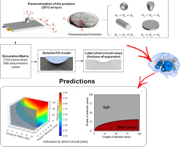
Flow-chart of the data-driven safety envelope using the ML algorithm. Figure adapted with permission from ref (324). Copyright 2019 Elsevier.

Figure 39

Schematic representation of the approach used by Severson et al. allowing to predict battery cycle life from only its first ∼100 cycles. Figure adapted with permission from ref (65). Copyright 2019 Springer.

Figure 40

(A) Schematic of the CLO system developed by Attia et al. (B) Example of the result showing the optimization time needed for different CLO protocols. Reprinted from Attia et al.^, Figure reproduced with permission from ref (338). Copyright 2020 Nature Publishing Group.

Figure 41

Overall framework of the proposed capacity estimation by Choi et al. Figure reproduced with permission from ref (326). Copyright 2019 IEEE.

Figure 42

Block diagram of the model migration by ref (355). Figure reproduced with permission from ref (355). Copyright 2009 Wiley.

Figure 43

Schematic overview of the scope of the work of Klass et al. Performance measures of an EV battery cell are determined and compared from real tests as well as from EV battery usage data via SVM-based models and virtual tests (I = current, U = voltage, T = temperature, SOC = state-of-charge, m = measured, c = calculated, h = hypothetical, e = estimated). Figure reproduced with permission from ref (368). Copyright 2014 Elsevier.

Figure 44

GP-ICE flow diagram by Richardson et al. The data used in these plots is only for illustration purposes. Figure reproduced with the authors permission from ref (377).

Figure 45

(a) Electrochemical thermal NN (ETNN) model structure and (b) NN detail by Feng et al. (a, b) Figure reproduced with permission from ref (383). Copyright 2020 Elsevier.

Figure 46

Architecture of the LSTM cell by Qu et al. Figure reproduced with permission from ref (328). Copyright 2019 IEEE.

Figure 47

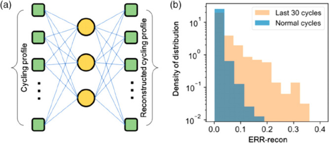
(a) Autoencoder anomaly detector for failure prediction: schematics of an autoencoder NN and (b) cycles before the last 30 and within the last 30 show distinct features indicated by the reconstruction error of the autoencoder. (a, b) Figure reproduced with permission from ref (386). Copyright 2019 Wiley.

Figure 48

Infographic on the ML methods recently used in the literature for applications to surrogate models, battery recycling/second life, and text mining, including the corresponding nature (calculated vs experimental data) of the employed databases.

Figure 49

Process flowchart for the creation of surrogate models from simulated data. Figure reproduced with permission from ref (408). Copyright 2018 IOPScience.

Figure 50

Graphical representation of the 1D device-scale simulation and multiscale model flowchart developed by Bao et al. The insert within the box enclosed by the dashed blue border reports the DNN scheme used for learning the relationship between flow-battery operating conditions and surface reaction uniformity. Figure adapted with permission from ref (23). Copyright 2020 Wiley.

Figure 51

Schematic representation of how the SVM-based approach proposed by Zhou et al. could assist the second life of EV battery for application as stationary applications. Figure adapted with permission from ref (416). Copyright 2020 Elsevier.

Figure 52

Overall process of text mining.

Figure 53

Percentages of LIB articles in which selected electrode and cell features were found through the text mining algorithm developed by El-Bousiydy et al. For the case of mass loading, porosity, and thickness, it was calculated as well how frequently those properties are reported as exact or approximate/range of values. Figure reproduced with permission from ref (20). Copyright 2021 Wiley.

Figure 54

Smart machines and humans working in strong synergy, a foreseeable future for AI in battery research for the coming years.

References

-
- https://www.ipcc.ch/sr15/ (accessed November 2020).
- Liu Z.; Ciais P.; Deng Z.; Lei R.; Davis S. J.; Feng S.; Zheng B.; Cui D.; Dou X.; Zhu B.; Guo R.; Ke P.; Sun T.; Lu C.; He P.; Wang Y.; Yue X.; Wang Y.; Lei Y.; Zhou H.; Cai Z.; Wu Y.; Guo R.; Han T.; Xue J.; Boucher O.; Boucher E.; Chevallier F.; Tanaka K.; Wei Y.; Zhong H.; Kang C.; Zhang N.; Chen B.; Xi F.; Liu M.; Bréon F. M.; Lu Y.; Zhang Q.; Guan D.; Gong P.; Kammen D. M.; He K.; Schellnhuber H. J. Near-Real-Time Monitoring of Global CO2 Emissions Reveals the Effects of the COVID-19 Pandemic. Nat. Commun. 2020, 11, 5172.10.1038/s41467-020-18922-7. - DOI - PMC - PubMed
- https://www.iea.org/data-and-statistics/charts/global-energy-related-co2... (accessed May 2021).
- https://www.iea.org/reports/global-ev-outlook-2021 (accessed May 2021).
Publication types
MeSH terms
LinkOut - more resources
Full Text Sources
Other Literature Sources