Circular RNA repertoires are associated with evolutionarily young transposable elements

Abstract

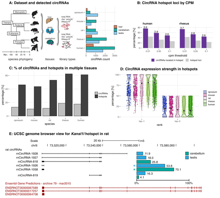
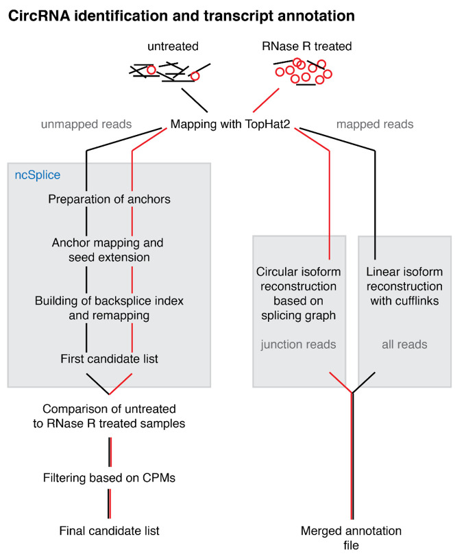
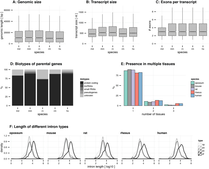
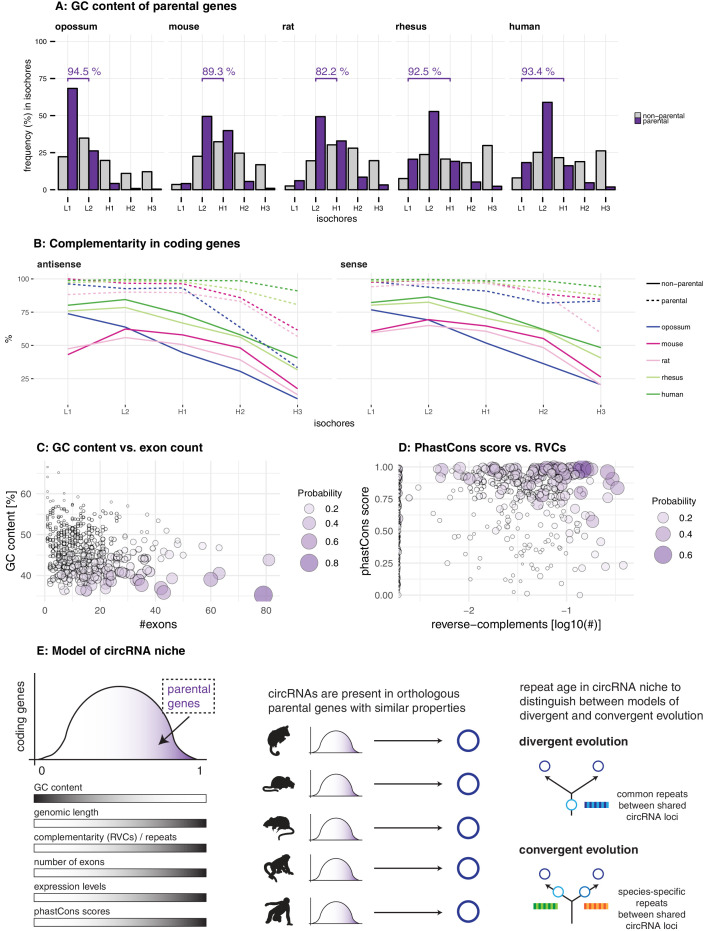
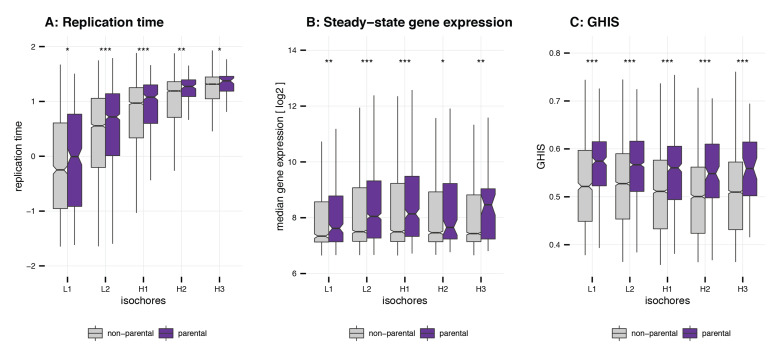
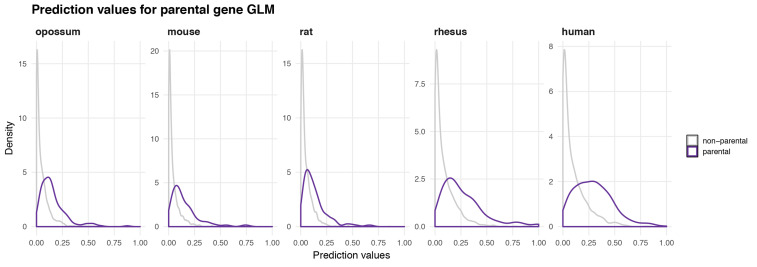
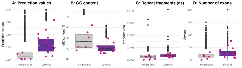
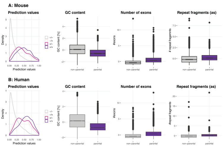
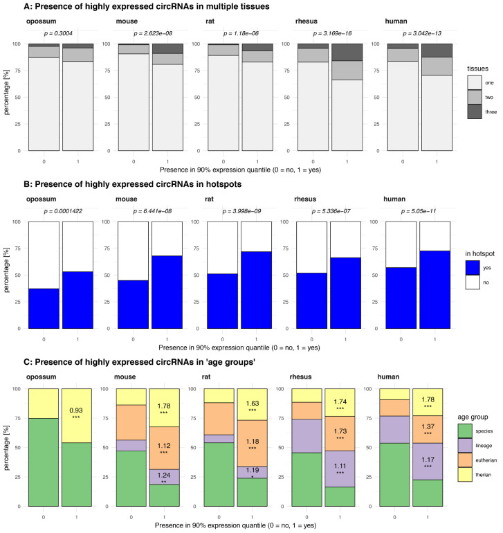
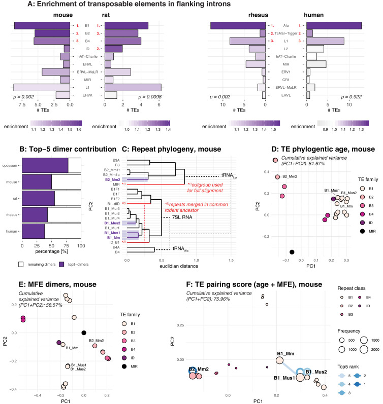
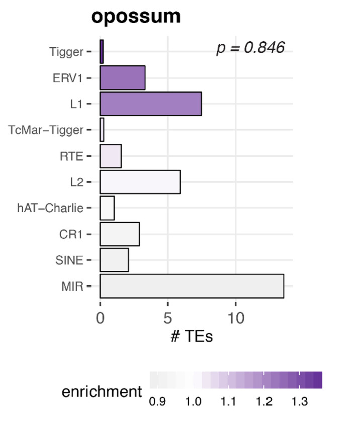
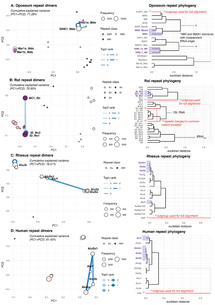
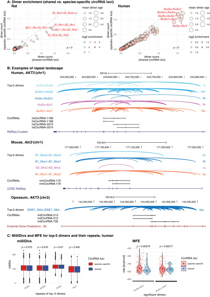
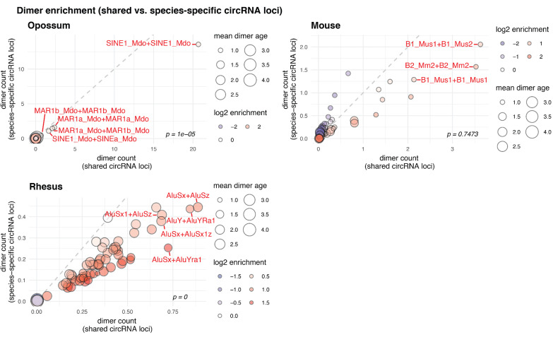
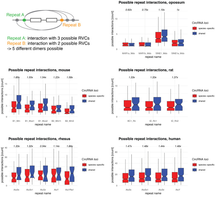
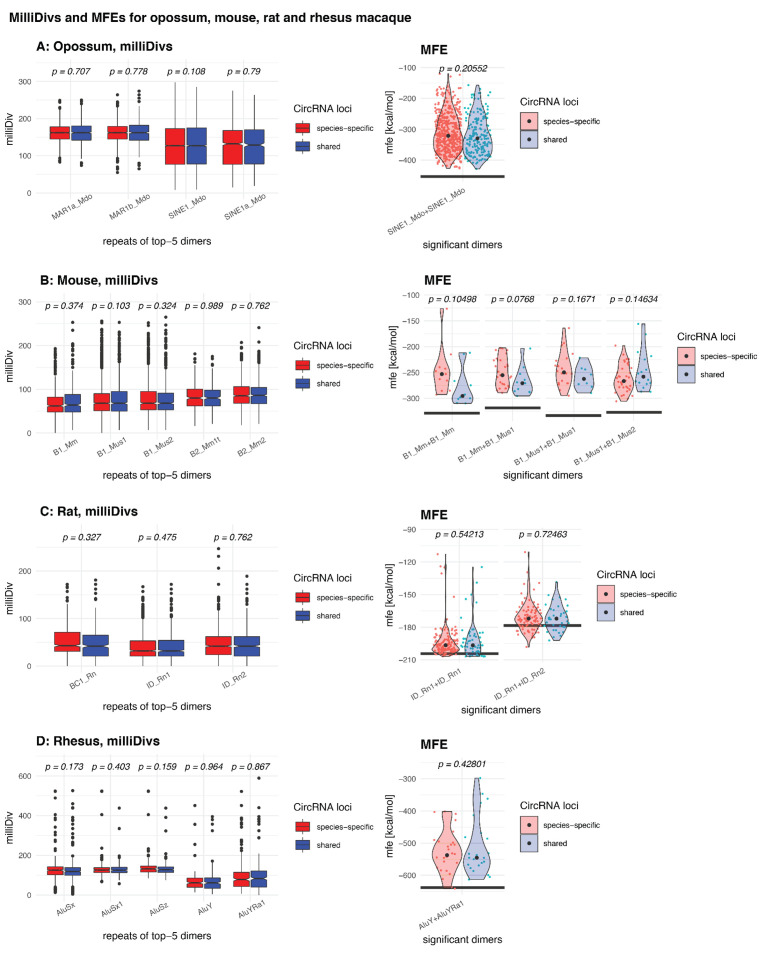
Circular RNAs (circRNAs) are found across eukaryotes and can function in post-transcriptional gene regulation. Their biogenesis through a circle-forming backsplicing reaction is facilitated by reverse-complementary repetitive sequences promoting pre-mRNA folding. Orthologous genes from which circRNAs arise, overall contain more strongly conserved splice sites and exons than other genes, yet it remains unclear to what extent this conservation reflects purifying selection acting on the circRNAs themselves. Our analyses of circRNA repertoires from five species representing three mammalian lineages (marsupials, eutherians: rodents, primates) reveal that surprisingly few circRNAs arise from orthologous exonic loci across all species. Even the circRNAs from orthologous loci are associated with young, recently active and species-specific transposable elements, rather than with common, ancient transposon integration events. These observations suggest that many circRNAs emerged convergently during evolution - as a byproduct of splicing in orthologs prone to transposon insertion. Overall, our findings argue against widespread functional circRNA conservation.

Keywords: circRNA; evolution; evolutionary biology; genetics; genomics; human; mammals; mouse; rat; rhesus macaque; splicing; transposons.

Figure 1.. Study design, samples, datasets, and characterisation of circRNA properties and hotspots.

(A) Phylogenetic tree of species analysed in this study and detected circRNAs. CircRNAs were identified and analysed in five mammalian species (opossum, mouse, rat, rhesus macaque, human) and three organs (liver, cerebellum, testis). Each sample was split and one half treated with RNase R to enrich BSJs. A dataset of high confidence circRNAs was established, based on the enrichment of BSJs in RNase R-treated over untreated samples. To the right of the panel, the total number of circRNAs for each species in liver (brown), cerebellum (green), and testis (blue) is shown. (B) CircRNA hotspot loci by CPM (human and rhesus macaque). The graph shows, in grey, the proportion (%) of circRNA loci that qualify as hotspots and, in purple, the proportion (%) of circRNAs that originate from such hotspots, at three different CPM thresholds (0.01, 0.05, 0.1). The average number of circRNAs per hotspot is indicated above the purple bars. (C) Number of circRNA hotspot loci found in multiple tissues. The graph shows the proportion (%) of circRNAs (light grey) and of hotspots (dark grey) that are present in at least two tissues. (D) Contribution of top-1 and top-2 expressed circRNAs to overall circRNA expression from hotspots. The plot shows the contribution (%) that the two most highly expressed circRNAs (indicated as top-1 and top-2) make to the total circRNA expression from a given hotspot. For each plot, the median is indicated with a grey point. (E) Example of the Kansl1l hotspot in rat. The proportion (%) for each detected circRNA within the hotspot and tissue (cerebellum = green, testis = blue) are shown. The strongest circRNA is indicated by an asterisk. rnCircRNA-819 is expressed in testis and cerebellum.

Figure 1—figure supplement 1.. Overview of the reconstruction pipeline.

Overview of the reconstruction pipeline. CircRNA identification and transcript reconstruction. Unmapped reads from RNA-seq data were remapped and analysed with a custom pipeline. The reconstruction of circRNA transcripts was based on the junction enrichment after RNase R treatment. Further details on the pipeline are provided in the Materials and methods.

Figure 1—figure supplement 2.. Mapping summary of RNA-seq reads.

Percentage of mapped, unmapped, multi-mapped and BSJ reads across all libraries in untreated and RNase R-treated conditions.

Figure 1—figure supplement 3.. General circRNA properties.

(A) Genomic size. The genomic size (bp) of circRNAs is plotted for all species. (B) Transcript size. The transcript size (nt) of circRNAs is plotted for all species. (C) Exons per transcript. The number of exons in circRNAs is plotted for all species. For panel A-C, outliers are not plotted (abbreviations: md = opossum, mm = mouse, rn = rat, rm = rhesus macaque, hs = human). (D) Biotypes of parental genes. For each species, the frequency (%) of different biotypes in the circRNA parental genes was assessed using the ensembl annotation. CircRNA loci that were not found in the annotation were marked as ‘unknown’. (E) Presence in multiple tissues. For each species, the frequency (%) of circRNAs detected in one, two, or three tissues is plotted. (F) Length of different intron types. Distribution of median intron length (log10-transformed) is plotted for different intron types in each gene. Abbreviations: np = non-parental, po = parental-outside of circRNA, pf = parental-flanking of circRNA, pi = parental-inside of circRNA.

Figure 1—figure supplement 4.. CircRNA hotspot loci by CPM (opossum, mouse, rat).

In grey, the proportion (%) of circRNA loci that qualify as hotspots and, in purple, the proportion (%) of circRNAs that originate from such hotspots, at three different CPM thresholds (0.01, 0.05, 0.1). The average number of circRNAs per hotspot is indicated above the purple bars.

Figure 2.. Evolutionary properties of circRNAs.

(A) CircRNA loci overlap between species. Upper panel: Schematic representation of the orthology definition used in our study. CircRNAs were collapsed for each gene, and coordinates were lifted across species. Lower panel: Number of circRNA loci that are species-specific (red) or circRNAs that arise from orthologous exonic loci of 1:1 orthologous genes (i.e. circRNAs sharing 1:1 orthologous exons) across lineages (purple) are counted. We note that in the literature, other circRNA ‘orthology’ definitions can be found, too. For example, assigning circRNA orthology simply based on parental gene orthology implies calling also those circRNAs ‘orthologous’ that do not share any orthologous exons, which directly argues against the notion of circRNA homology; that is, a common evolutionary origin (see Figure 2—figure supplement 1A). Overall, the orthology considerations we applied largely follow the ideas sketched out in Patop et al., 2019. (B) Distribution of phastCons scores for different exon types. PhastCons scores were calculated for each exon using the conservation files provided by ensembl. PhastCons scores for non-parental exons (grey), exons in parental genes, but outside of the circRNA (pink) and circRNA exons (purple) are plotted. The difference between circRNA exons and non-parental exons that can be explained by parental non-circRNA exons is indicated above the plot. (C) Mean tissue frequency of different exon types in parental genes. The frequency of UTR exons (grey), non-UTR exons outside of the circRNA (pink) and circRNA exons (purple) that occur in one, two, or three tissues was calculated for each parental gene. (D) Distribution of splice site amplitudes for different exon types. Distribution of median splice site GC amplitude (log2-transformed) is plotted for different exon types (np = non-parental, po = parental, but outside of circRNA, pi = parental and inside circRNA). Red vertical bars indicate values at which exon and intron GC content would be equal. (E) Different evolutionary models explaining the origins of overlapping circRNA loci.

Figure 2—figure supplement 1.. CircRNA loci overlap between species.

(A) Upper panel: The presence of circRNA in multiple species can be identified on the gene level (=‘parental gene’), based on the location of the circRNA within the gene (=‘circRNA locus’) or the overlap of the first and last exons of the circRNA (=‘start/stop exon’). Depending on the chosen stringency, the number of circRNA loci present in multiple species varies. For example: when considering the parental gene level (shown to the left), all four circRNAs depicted in the hypothetical example of this figure (circRNA-A.1, circRNA-A.2, circRNA-B.1, and circRNA-B.1) are located in the same orthologous locus. In contrast, when looking at the start and stop exons (right), only two circRNAs (circRNA-A.1 and circRNA-B.1) are generated from the same orthologous locus, whereas circRNA-A.2 and circRNA-B.2 - previously classified as ‘orthologous’ – are now found in different loci and labeled as species-specific. Depending on the classification, the number of shared circRNA loci thus differs and may influence the interpretation of results. Lower panel: For each classification, orthology clusters were counted and grouped by their overlap (in purple when present in primates, rodents, eutherians or therians; in red when species-specific). Please note that in our study, we apply the definition shown in the middle panels (which are identical to main Figure 2A) that considers exon overlap as relevant. (B) Figure shows the loss of shared circRNA loci (based on ‘circRNA locus’ definition) by adding additional species to the classical mouse-human comparison. All comparisons are made with mouse as reference to which the other loci are compared. The reduction of loci (%) by adding additional species is indicated below each figure.

Figure 2—figure supplement 2.. Amplitude correlations.

Plotted is the correlation (Spearman’s rho) between the amplitude and the GC content of introns (light brown) and exons (dark brown). Abbreviations: np = non-parental, po = parental, outside of circRNA, pi = parental, inside of circRNA.

Figure 3.. Characterisation of circRNA parental gene properties.

(A) GC content of parental genes. Coding genes were classified into L1-H3 based on their GC content, separately for non-parental (grey) and parental genes (purple). The percentage of parental genes in L1-L2 (opossum, mouse, rat) and L1-H1 (rhesus macaque, human) is indicated above the respective graphs. (B) Complementarity in coding genes. Each coding gene was aligned to itself in sense and antisense orientation using megaBLAST. The proportion of each gene involved in an alignment was calculated and plotted against its isochore. (C-D) Examples of parental gene predictors for linear regression models. A generalised linear model (GLM) was fitted to predict the probability of the murine coding gene to be parental, whereby x- and y-axis represent the strongest predictors. Colour and size of the discs correspond to the p-values obtained for 500 genes randomly chosen from all mouse coding genes used in the GLM. (E) Model of circRNA niche.

Figure 3—figure supplement 1.. Replication time, gene expression steady-state levels and GHIS of human parental genes.

(A) Replication time of parental genes. Values for the replication time were used as provided in Koren et al., 2012. They were normalised to a mean of 0 and a standard deviation of 1. Differences between non-parental genes (n_total = 18134) and parental genes (n_total = 2058) were assessed by a one-tailed Mann-Whitney U test. (B) Gene expression steady-state levels of parental genes. Mean steady-state expression levels were used as provided in Pai et al., 2012. Differences between non-parental genes (n_total = 14414) and parental genes (n_total = 2058) were assessed by a one-tailed Mann-Whitney U test. (C) GHIS of parental genes. GHIS was used as provided in Steinberg et al., 2015. Differences between non-parental genes (n_total = 17438) and parental genes (n_total = 1995) were assessed by a one-tailed Mann-Whitney U test. (Note C-D: Outliers for all panels were removed prior to plotting. Significance levels: '***' < 0.001, '**' < 0.01, '*' < 0.05, 'ns' >= 0.05).

Figure 3—figure supplement 2.. Distribution of prediction values for non-parental and parental circRNA genes.

The density of predicted values for non-parental (grey) and parental (purple) genes is plotted for each species based on the predictors identified by the GLM in each species.

Figure 3—figure supplement 3.. Properties of ‘functional circRNAs’ from literature.

(A) Prediction values of linear regression model for human circRNA parental and non-parental genes as previously defined (Materials and methods). Functional circRNAs as described in Chen, 2020 are plotted in pink on top of the boxplot and are separated by whether they are in a non-parental or parental gene. (B-D) GC content, repeat fragments (in antisense, normalised by genomic length of parental gene) and number of exons for human non-parental and parental circRNA genes; values for functional circRNAs are plotted in pink. Parental genes of functional circRNAs listed in Chen, 2020, which were identified in our study: SHPRH, ZNF609, GCN1L1, HIPK2, HIKP3, ZNF91, BIRC6, FOXO3, MBNL1, ASAP1, PAN3, SMARCA5, ITCH.

Figure 3—figure supplement 4.. Validation of parental gene GLM on Werfel et al. dataset.

(A) Mouse. To assess the parental gene properties identified by this study, the generalised model was used to predict circRNA parental genes on data from an independent study. The density plot ‘Prediction values’ shows the predicted values for non-parental genes in both datasets (Werfel et al., 2016 and data from this publication, n = 11963, in grey and labeled as -/-), parental genes only present in the Werfel dataset (n = 2843, light pink, labeled as -/+), parental genes only present in this study’s underlying dataset (n = 210, dark pink, labeled as +/-) and parental genes that were present in both datasets (n = 638, purple, labeled as +/+). The plots ‘GC content’, ‘Number of exons’ and ‘Repeat fragments (as)’ (the latter normalised by the genomic length of the parental gene) show the properties of circRNA parental genes (highlighted in purple) as identified by Werfel et al. (B) Human. Same plot outline as for mouse. The number of non-parental genes in both datasets is n = 10591; 2724 parental genes are only present in the Werfel dataset and 356 parental genes only in our dataset. The overlap between both datasets is n = 1666.

Figure 3—figure supplement 5.. Properties of highly expressed circRNAs.

(A) Presence of highly expressed circRNAs in multiple tissues. Plot shows the percentage (%) of circRNAs from the 90% expression quantile (n_opossum = 158, n_mouse = 156, n_rat = 217, n_rhesus = 340, n_human = 471), which is present in one, two or three of the tissues analysed compared to circRNAs outside the 90% expression quantile. For each species, distributions were compared using Fisher’s exact test, p-values are shown above each barplot. (B) Presence of highly expressed circRNAs in hotspots. Plot shows the percentage (%) of circRNAs from the 90% expression quantile, which is found in a hotspot compared to circRNAs outside the 90% expression quantile. For each species, distributions were compared using Fisher’s exact test, p-values are shown above each barplot. (C) Presence of highly expressed circRNAs in ‘age groups’. Plot shows the percentage (%) of circRNAs from the 90% expression quantile, which is present in different ‘age groups’ compared to circRNAs outside the 90% expression quantile. Age groups were defined as whether circRNA is species-specific (age = 1), lineage-specific (age = 2), eutherian (age = 3) or shared across all therian species (age = 4). Log-odds ratio and significance levels (significance levels based on p-value: ‘***’ < 0.001, ‘**’ < 0.01, ‘*’ < 0.05, ‘ns’ >= 0.05) were calculated using a generalised linear model (see Supplementary file 10) and are shown for the respective age groups and species.

Figure 4.. Analysis of the repeat landscape of circRNA parental genes.

(A) Enrichment of TEs in flanking introns for mouse, rat, rhesus macaque and human. The number of TEs was quantified in both intron groups (circRNA flanking introns and length- and GC-matched control introns). Enrichment of TEs is represented by colour from high (dark purple) to low (grey). The red numbers next to the TE name indicate the top-3 enriched TEs in each species. Enrichment was assessed using a Wilcoxon Signed Rank Test; p-values are indicated at the bottom of each plot. (B) Top-5 dimer contribution. The graph shows the proportion of top-5 dimers (purple) vs. other, remaining dimers (white) to all predicted dimers in flanking introns. Top-5 dimers thus account for 78, 50, 55, 43, and 38% of all dimers in opossum, mouse, rat, rhesus macaque and human, respectively. (C) Phylogeny of mouse TEs. Clustal-alignment based on consensus sequences of TEs. Most recent TEs are highlighted. (D) PCA for phylogenetic age of mouse TE families. PCA is based on the clustal-alignment distance matrix for the reference sequences of all major SINE families in mouse with the MIR family used as an outgroup. TEs present in the top-5 dimers are labelled. (E) PCA based on binding affinity of mouse TE families. PCA is based on the minimal free energy (MFE) for all major SINE families in mouse with the MIR family used as an outgroup. TEs present in the top-5 dimers are labelled. (F) PCA for TE pairing score of mouse dimers. PCA is based on a merged and normalised score, taking into account binding strength of the dimer structure (=MFE) and phylogenetic distance. Absolute frequency of TEs is visualised by circle size. TEs present in the five most frequent dimers (top-5) are highlighted by blue lines connecting the two TEs engaged in a dimer (most frequent dimer in dark blue = rank 1). If the dimer is composed of the same TE family members, the blue line loops back to the TE (=blue circle).

Figure 4—figure supplement 1.. Enrichment of transposable elements in flanking introns for opossum.

The number of transposable elements was quantified in both intron groups (circRNA flanking introns and length- and GC-matched control introns). Enrichment of transposable elements is represented by colour from high (dark purple) to low (grey). The frequency distributions of TEs in background and flanking introns were compared using a Wilcoxon Signed Rank Test; p-value is shown in the upper right corner.

Figure 4—figure supplement 2.. PCA and phylogeny of opossum, rat, rhesus macaque, and human repeat dimers.

(A) Opossum. Panel A shows the PCA for dimer clustering based on a merged and normalised score, taking into account binding phylogenetic distance, binding capacity of TEs to each other and absolute frequency. Absolute frequency is also represented by circle size. The top-ranked dimers are indicated. Circles around the discs represent cases where the TE binds to itself. Furthermore, a phylogeny of opossum transposable elements is shown, the top-5 dimers are highlighted with purple shading. Phylogenetic trees are based on multiple alignments with Clustal-Omega. Several TE families have independent origins, which cannot be taken into account with Clustal-Omega. These cases are indicated by a grey, dotted line and TE origins – if known – have been manually added. We deemed this procedure sufficiently precise, given that the aim was to only visualise the general relationship of TEs. TEs used as outgroups, as well TEs that merged are indicated with a red line. (B-D) Same analysis as in Panel A, but for rat, rhesus macaque, and human, respectively.

Figure 5.. Repeat analysis and dimer potential of shared and species-specific parental genes.

(A) Dimer enrichment in shared vs. species-specific repeats in rat and human (see Figure 5—figure supplement 1 for other species). The frequency (number of detected dimers in a given parental gene), log2-enrichment (shared vs. species-specific) and mean age (defined as whether repeats are species-specific: age = 1, lineage-specific: age = 2, eutherian: age = 3, therian: age = 4) of the top-100 most frequent and least frequent dimers in parental genes with shared and species-specific circRNA loci in rat and human were analysed. The frequency is plotted on the x- and y-axis, point size reflects the age and point colour the enrichment (blue = decrease, red = increase). Based on the comparison between shared and species-specific dimers (using a Wilcoxon Signed Rank Test), the top-5 dimers defined by frequency and enrichment are highlighted and labelled in red. (B) Species-specific dimer landscape for the Akt3 gene in human, mouse and opossum. UCSC genome browser view for the parental gene, circRNAs and top-5 dimers (as defined in panel B). Start and stop positions of each dimer are connected via an arc. Dimers are grouped by composition represented by different colours, the number of collapsed dimers is indicated to the right-side of the dimer group. Only dimers that start before and stop after a circRNAs are shown as these are potentially those that can contribute to the hairpin structure. The human Akt3 gene possesses two circRNA clusters. For better visualisation, only the upstream cluster is shown. (C) Degradation rates (MilliDivs) and minimal free energy (MFE) for top-5 dimers in human. MilliDiv values for all repeats composing the top-5 dimers (defined by their presence in all parental genes) were compared between parental genes of species-specific (red) and shared (blue) circRNA loci in human (see Figure 5—figure supplement 3 for other species). A Wilcoxon Signed Rank Test was used to compare dimers between parental genes with shared and species-specific circRNA loci, with p-values plotted above the boxplots. MFE values were compared between the least degraded dimers in parental genes of species-specific (red) and shared (blue) circRNA loci. MFE values were calculated using the genomic sequences of all top-5 dimers. For each parental gene, the least degraded dimer (based on its mean milliDiv value) was then chosen which let to a strong enrichment of only a subset of the top-5 dimers (in this case AluSx+AluY and AluSx1+AluY). If enough observations for a statistical test were present, the two distributions (shared/species-specific) were compared using a Student’s t-Test and plotted as violin plots with p-values above the plot.

Figure 5—figure supplement 1.. Contribution of species-specific repeats to the formation of shared circRNA loci.

Dimer enrichment in shared and species-specific repeats in opossum, mouse and rhesus macaque. The frequency (number of detected dimers in a given parental gene), log2-enrichment (shared vs. species-specific) and mean age (defined as whether repeats are species-specific: age = 1, lineage-specific: age = 2, eutherian: age = 3, therian: age = 4) of the top-100 most frequent and least frequent dimers in parental genes with shared and species-specific circRNA loci in opossum, mouse and rhesus macaque were analysed and compared with a Wilcoxon Signed Rank Test. Frequencies are plotted on the x- and y-axis, point size reflects the age and point colour the enrichment (blue = decrease, red = increase). Based on the comparison between shared and species-specific dimers, the top-5 dimers defined by frequency and enrichment are highlighted and labelled in red.

Figure 5—figure supplement 2.. Repeat interaction landscape in shared vs. species-specific circRNA loci.

Upper left: graphical representation of possible repeat interactions (=dimers that can be formed) across RVCs. Afterwards: Frequency distribution of possible interactions of a given repeat (from the top-5 dimers, based on Figure 5A and Figure 5—figure supplement 1) in parental genes of species-specific (red) and shared (blue) circRNA loci in opossum, mouse, rat, rhesus macaque, and human. The enrichment of possible interactions (shared vs. species-specific, based on each distribution’s median) is indicated above each plot.

Figure 5—figure supplement 3.. MilliDivs and MFE for dimers in shared and species-specific circRNA loci.

Left panel of each species: MilliDiv values were compared between parental genes of species-specific (red) and shared (blue) circRNA loci using a Student’s t-Test (alternative = ‘less’) with corresponding p-values plotted above each boxplots. Since dimers are composed of two repeats, the mean milliDiv value between both repeats was taken. Right panel of each species: Violin Plots depicting the minimal free energy (MFE) of genomic sequences for dimers in species-specific (red) and shared (blue) circRNA loci. For each gene, the ‘least degraded dimer’ was chosen to calculate its MFE value leading to a strong enrichment of only a few of the top-5 dimers (see Materials and methods). The ‘maximum’ MFE possible, which is based on the dimer formed by each TE’s reference sequence (downloaded from RepBase [Bao et al., 2015]), is depicted with a grey line below each pair of violin plots. Each distribution’s median is indicated with a grey point. MFE values between species-specific and shared circRNA loci were compared with a Student’s t-Test; corresponding p-values are indicated above each pair of violin plots.

References

1. Alhasan AA, Izuogu OG, Al-Balool HH, Steyn JS, Evans A, Colzani M, Ghevaert C, Mountford JC, Marenah L, Elliott DJ, Santibanez-Koref M, Jackson MS. Circular RNA enrichment in platelets is a signature of transcriptome degradation. Blood. 2016;127:e1–e11. doi: 10.1182/blood-2015-06-649434. - DOI - PMC - PubMed
1. Amit M, Donyo M, Hollander D, Goren A, Kim E, Gelfman S, Lev-Maor G, Burstein D, Schwartz S, Postolsky B, Pupko T, Ast G. Differential GC content between exons and introns establishes distinct strategies of splice-site recognition. Cell Reports. 2012;1:543–556. doi: 10.1016/j.celrep.2012.03.013. - DOI - PubMed
1. Ashwal-Fluss R, Meyer M, Pamudurti NR, Ivanov A, Bartok O, Hanan M, Evantal N, Memczak S, Rajewsky N, Kadener S. circRNA biogenesis competes with pre-mRNA splicing. Molecular Cell. 2014;56:55–66. doi: 10.1016/j.molcel.2014.08.019. - DOI - PubMed
1. Athanasiadis A, Rich A, Maas S. Widespread A-to-I RNA editing of Alu-containing mRNAs in the human transcriptome. PLOS Biology. 2004;2:e391. doi: 10.1371/journal.pbio.0020391. - DOI - PMC - PubMed
1. Bachmayr-Heyda A, Reiner AT, Auer K, Sukhbaatar N, Aust S, Bachleitner-Hofmann T, Mesteri I, Grunt TW, Zeillinger R, Pils D. Correlation of circular RNA abundance with proliferation--exemplified with colorectal and ovarian Cancer, idiopathic lung fibrosis, and normal human tissues. Scientific Reports. 2015;5:8057. doi: 10.1038/srep08057. - DOI - PMC - PubMed
Publication types