The three major axes of terrestrial ecosystem function

Abstract

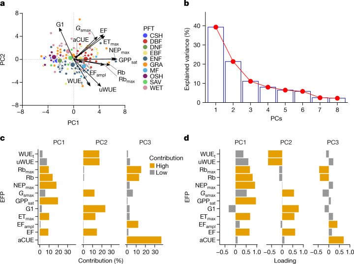
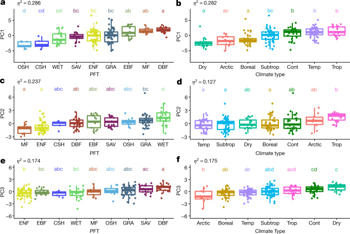
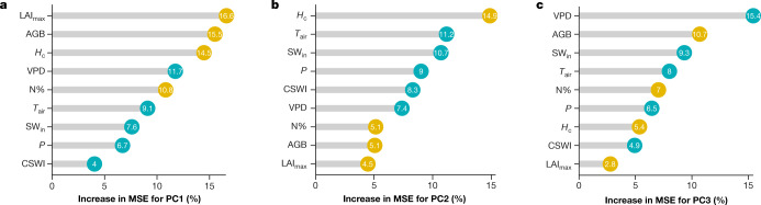
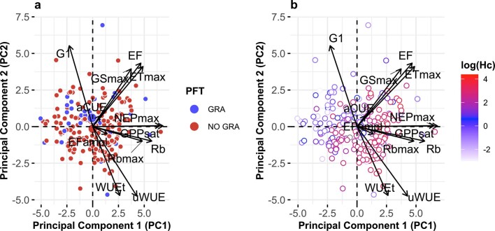
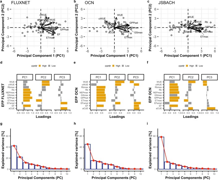
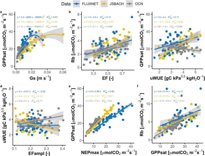
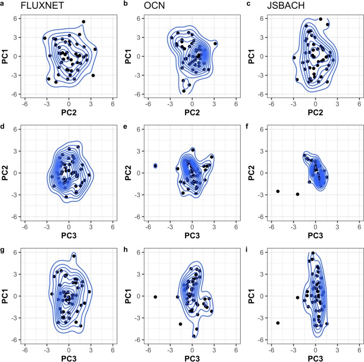
The leaf economics spectrum^1,2 and the global spectrum of plant forms and functions³ revealed fundamental axes of variation in plant traits, which represent different ecological strategies that are shaped by the evolutionary development of plant species². Ecosystem functions depend on environmental conditions and the traits of species that comprise the ecological communities⁴. However, the axes of variation of ecosystem functions are largely unknown, which limits our understanding of how ecosystems respond as a whole to anthropogenic drivers, climate and environmental variability^4,5. Here we derive a set of ecosystem functions⁶ from a dataset of surface gas exchange measurements across major terrestrial biomes. We find that most of the variability within ecosystem functions (71.8%) is captured by three key axes. The first axis reflects maximum ecosystem productivity and is mostly explained by vegetation structure. The second axis reflects ecosystem water-use strategies and is jointly explained by variation in vegetation height and climate. The third axis, which represents ecosystem carbon-use efficiency, features a gradient related to aridity, and is explained primarily by variation in vegetation structure. We show that two state-of-the-art land surface models reproduce the first and most important axis of ecosystem functions. However, the models tend to simulate more strongly correlated functions than those observed, which limits their ability to accurately predict the full range of responses to environmental changes in carbon, water and energy cycling in terrestrial ecosystems^7,8.

Fig. 1. Key dimensions of multivariate space of terrestrial ecosystem functions.

a, Biplot resulting from the PCA. Different colours of the points represent different plant functional types (PFTs): CSH (closed shrublands); DBF (deciduous broadleaved forest); DNF (deciduous needleleaf forests); EBF (evergreen broadleaved forest); ENF (evergreen needleleaf forest); GRA (grasslands); MF (mixed forest); OSH (open shrublands); SAV (savannah); and WET (wetlands). Bigger points represent the centroid of the distribution for each PFT. b, Explained variance for each principal component. c, d, Bar plots of the contribution (c) and loading (d) of each ecosystem functional property (EFP) to each principal component. Orange bars represent the loadings and the contributions that are considered significant (Supplementary Information 2).

Fig. 2. Distribution of plant functional types and climate types along the principal components (PC1–PC3).

a, c, e, Plant functional types (PFTs). b, d, f, Climate types. Letters represent statistically significant differences in the average PCs (Tukey’s HSD test, P < 0.05), such that groups not containing the same letter are different. The effect size of the one-way ANOVA (η²) is reported (n = 203 sites). In the box plots the central line represents the mean; the lower and upper box limits correspond to the 25th and 75th percentiles and the upper (lower) whiskers extend to 1.5 (−1.5) times the interquartile range, respectively. Colours indicate different climate types and PFTs (cont, continental; subtrop, subtropical; temp, temperate; trop, tropical; PFT definitions are as in Fig. 1).

Fig. 3. Importance of climate and vegetation properties.

a–c, Predictive relative importance for PC1 (a), PC2 (b) and PC3 (c). Numbers in the circles represent the percentage increase in mean squared error (MSE). Yellow circles represent vegetation structural variables; light blue circles represent climate variables.

Extended Data Fig. 1. Map of the 203 FLUXNET sites used in this analysis.

Colours represent different plant functional types according to the IGBP classification. IGBP classes are: CSH (close shrublands); DBF (deciduous broadleaved forest), DNF (deciduous needleleaf forests), EBF (evergreen broadleaved forest), ENF (evergreen needleleaf forest), GRA (grasslands), MF (mixed forest), OSH (open shrublands), SAV (savannah), and WET (wetlands). The map was generated with the ggplot2 R package. The shape files used to create the maps were downloaded from https://github.com/ngageoint/geopackage-js.

Extended Data Fig. 2. FLUXNET sites used in the analysis plotted in the precipitation–temperature space.

The background represent climate space of the major biomes according to Whittaker and further modifications. Biomes are defined as function of the mean annual temperature and mean annual precipitation (MAP). The figure is modified from Liu et al., using the code available in git (https://github.com/kunstler/BIOMEplot).

Extended Data Fig. 3. Distribution of the selected FLUXNET sites within the climate types.

Climate types were defined according to Köppen-Geiger classification as follow: Tropical (Aw, Af, Am), Dry (BSh, BSk, BWh), Temperate (Cfb), Sub-Tropical (Cfa, Csa, Csb, Cwa), Temperate/Continental Hot (Dfa, Dfb, Dwa, Dwb, Dwc), Arctic (ET)], and Boreal (Dfc, Dsc).

Extended Data Fig. 4. Results of the relative importance analysis conducted with the Random Forest and partial dependence.

See ‘Predictive variable importance’ in Methods. The slopes of the partial dependence plot indicate the sensitivity of the response (PCs) to the specific predictor. The out-of-bag cross-validation leads to predictive explained variance of 56.76% for PC1, 30.24% for PC2, and 20.41% for PC3. The portion of unexplained variance might be related to missing leaf traits predictor such as leaf mass per area or phenological traits. The partial dependence plots of all variables are shown: top panels for PC1 (a–e), middle panels for PC2 (f–l), and bottom panels for PC3 (m–q). The blue lines represent the locally estimated scatterplot (LOESS) smoothing of the partial dependence. Tick marks in the x axis represent the minimum, maximum and deciles of the variable distribution.

Extended Data Fig. 5. Map of FLUXNET sites colour-coded for the value of PC1 and PC2.

a, PC1. b, PC2. The map of the PC1 shows the areas of the globe with high productivity (positive values of PC1 in the temperate areas, Eastern North America, Eastern Asia, and Tropics), and areas characterized by lower productivity (Semi-arid regions, high latitude and Mediterranean ecosystems). The map of the PC2 shows the gradient of evaporative fraction and the spatial patterns of water use efficiency. This PC2 runs from sites with a high evaporative fraction (i.e. available energy is dissipated preferentially to evaporated or transpired water), high surface conductance, and low water use efficiency (positive PC2 values), to water limited sites (i.e. low evaporative fraction where available energy is mainly dissipated by sensible heat) that also show higher water-use efficiency (negative PC2 values). The maps were generated with the ggplot2 R package. The shape files used to create the maps were downloaded from https://github.com/ngageoint/geopackage-js.

Extended Data Fig. 6. Biplot resulting from the principal component analysis.

Plot as in Fig. 1. In panel a, points are colour-coded by grass vs. non-grass classes. In panel b, the points are colour-coded according to the logarithm of vegetation height. From these results we conclude that there is not a clear cluster in the biplot for grass and non-grass vegetation. In fact, in Extended Data Fig. 6a, the sites do not cluster according to the designation to grasslands or not, but there is a clear gradient as a function of the vegetation height (Extended Data Fig. 6b).

Extended Data Fig. 7. Comparing observed and modelled global ecosystem functional trade-offs.

PCA for a subset of 48 FLUXNET sites mainly distributed in temperate and boreal regions and 2 different land surface models (Supplementary Table 1). The left column is FLUXNET, the centre column is OCN, and the right column is JSBACH. Panels a, b, c: the biplot resulting from the PCA. Panels d, e, f, bar plot of the loading of each ecosystem functional property to each principal component. Orange bars represent the loadings that are selected as significant and with high contribution (Supplementary Information 2). Panels g, h, i report the variance explained by each principal component. EFP acronym list: apparent carbon-use efficiency (aCUE), evaporative fraction (EF), amplitude of EF (EF_ampl), maximum evapotranspiration (ET_max), gross primary productivity at light saturation (GPP_sat), maximum surface conductance (G_smax), maximum net ecosystem productivity (NEP_max), maximum and mean basal ecosystem respiration (Rb_max and Rb, respectively), and growing season underlying water-use efficiency (uWUE). Note that the PCA results for FLUXNET (panels a, d, g) are different from Fig. 1 because here we use the subset of 48 sites used for the modelling analysis.

Extended Data Fig. 8. Pairwise relationship between some key ecosystem functional properties derived from FLUXNET, and modelled with JSBACH and OCN.

n = 48 sites; see Supplementary Table 1. The grey areas represent the 95% confidence interval of the linear and nonlinear regression. Overall the correlation between modelled functions is larger than in the observations. Acronym list: evaporative fraction (EF), amplitude of EF (EF_ampl), gross primary productivity at light saturation (GPP_sat), maximum surface conductance (G_s), maximum net ecosystem productivity (NEP_max), basal ecosystem respiration (Rb), and growing season underlying water-use efficiency (uWUE).

Extended Data Fig. 9. Representation of the 2D ecosystem functional properties space derived from FLUXNET observations and land surface model runs (OCN, JSBACH).

The points represent the principal component (PC) value calculate for each site. The contour lines are computed using a 2D kernel density estimates. The contour lines show the area occupied by ecosystem functional properties and its boundary that, according to the results of the analysis, are set by vegetation characteristics (PC1), water availability, abiotic limitations, and vegetation height (PC2), and above-ground biomass, foliar nitrogen and atmospheric aridity (PC3). The areas computed for FLUXNET are wider than for the models, particularly for PC2 and PC3. This means that ecosystem functional properties as simulated by models are more constrained than for the observations.

Extended Data Fig. 10. Evaluation of above-ground biomass satellite products against FLUXNET observation.

n = 71. We evaluated the three above-ground biomass (AGB, t DM ha⁻¹) products derived from the GlobBiomass dataset as reported in the Method section. From the product at its original resolution (100 x 100 m) we extracted the 95th percentile of the estimated AGB in 5 by 5 grid cell windows (AGB5x5, panel a with all sites, and panel b with the grasslands excluded) centered around the location of the FLUXNET sites used for the evaluation. Further, we extracted the median in 3 by 3 and 5 by 5 grid cells centered around the location of the FLUXNET site (panels c and d). Total above-ground biomass observations were gathered from the BADM dataset downloaded from the AMERIFLUX network and from the FLUXNET LaThuile release. Only data with the clear indication of the unit of AGB expressed in in dry matter (t DM ha⁻¹) were retained for the analysis. Results show that the median of the 5 by 5 grid cell window (panel c) is the best extraction method to characterize AGB at the FLUXNET sites, and therefore retained for further analysis. Adjusted determination coefficient (R²), linear regression function, and p-value calculated with the F-test are also reported.

References

1. Wright IJ, et al. The worldwide leaf economics spectrum. Nature. 2004;428:821–827. doi: 10.1038/nature02403. - DOI - PubMed
1. Reich PB, Walters MB, Ellsworth DS. From tropics to tundra: global convergence in plant functioning. Proc. Natl Acad. Sci. USA. 1997;94:13730–13734. doi: 10.1073/pnas.94.25.13730. - DOI - PMC - PubMed
1. Díaz S, et al. The global spectrum of plant form and function. Nature. 2016;529:167–171. doi: 10.1038/nature16489. - DOI - PubMed
1. Bruelheide H, et al. Global trait–environment relationships of plant communities. Nat. Ecol. Evol. 2018;2:1906–1917. doi: 10.1038/s41559-018-0699-8. - DOI - PubMed
1. Manning P, et al. Redefining ecosystem multifunctionality. Nat. Ecol. Evol. 2018;2:427–436. doi: 10.1038/s41559-017-0461-7. - DOI - PubMed
Publication types