Quantitative magnetic resonance imaging and tumor forecasting of breast cancer patients in the community setting

Abstract

This protocol describes a complete data acquisition, analysis and computational forecasting pipeline for employing quantitative MRI data to predict the response of locally advanced breast cancer to neoadjuvant therapy in a community-based care setting. The methodology has previously been successfully applied to a heterogeneous patient population. The protocol details how to acquire the necessary images followed by registration, segmentation, quantitative perfusion and diffusion analysis, model calibration, and prediction. The data collection portion of the protocol requires ~25 min of scanning, postprocessing requires 2-3 h, and the model calibration and prediction components require ~10 h per patient depending on tumor size. The response of individual breast cancer patients to neoadjuvant therapy is forecast by application of a biophysical, reaction-diffusion mathematical model to these data. Successful application of the protocol results in coregistered MRI data from at least two scan visits that quantifies an individual tumor's size, cellularity and vascular properties. This enables a spatially resolved prediction of how a particular patient's tumor will respond to therapy. Expertise in image acquisition and analysis, as well as the numerical solution of partial differential equations, is required to carry out this protocol.

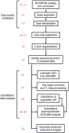
Fig. 1 ∣. Overview of the protocol.

Each panel contains summary keywords for each section. The procedure has five major sections: defining the patient population (Step 1, not shown), image acquisition (Steps 2-9), data analysis (Steps 10-25), mapping imaging data to the mathematical model (Steps 26-36), and tumor forecasting (Steps 37-40). Each section of the procedure focuses on specific areas of the protocol, and each section can be adapted for alternative investigations or used independently given specific circumstances in other studies. For example, the image acquisition section can be adapted for MRI studies in other organs. Also, given imaging data that are already acquired and analyzed, the mapping and forecasting sections can be applied. Note that informed consent must be obtained from all subjects. DCE-MRI, dynamic contrast-enhanced MRI; DW-MRI, diffusion-weighted MRI.

Fig. 2 ∣. Timeline of MRI acquisition with an example standard-of-care NAT regimen for triple-negative breast cancer consisting of two therapeutic regimens.

a, Example NAT regimen only. b, Example regimen with the protocol’s calibration and prediction strategy. For a and b, wide arrows indicate the first dose and start of each cycle (i.e., the administration of a single drug or combination of drugs over a designated period of time, typically 2–4 weeks), while the narrow arrows indicate any additional doses within each cycle. For the first regimen, red arrows represent combination doxorubicin and cyclophosphamide (typically consisting of four cycles where drugs are administered as single doses separated by 2 weeks). For the second regimen, blue arrows represent paclitaxel (typically consisting of four cycles where therapy is administered every week with each cycle lasting 3 weeks—small arrows represent the additional doses). Some patients are treated with carboplatin in combination with paclitaxel, where carboplatin is administered during the first week of each paclitaxel cycle only (wide blue arrows). After NAT is complete, patients undergo surgery as part of their standard of care to determine pathological response. The protocol has MRI data collected prior to and just after the first cycle of each therapeutic regimen.

Fig. 3 ∣. FCM clustering to generate a tumor ROI.

Depicted is the sagittal cross section of a breast for the average DCE-MRI data for one patient (all panels). For the middle panel, a manually drawn ROI is shown, which identifies a conservative bounding polygon for the tumor. The right panel depicts the resulting ROI generated from the FCM algorithm within the manually drawn bounding polygon. Informed consent was obtained from this patient.

Fig. 4 ∣. Comparison of intervisit registration results with and without tumor ROI penalties incorporated into the registration scheme.

a, Target image (scan 2, defined in Fig. 2). b, ‘Moving’ image to be deformed/shifted to align to the target image (scan 3). In b, the moving image’s tumor ROI is indicated by a black outline. c, Result of registering the moving image to the target image using the approach described in Steps 27-31 of the text (i.e., rigid + nonrigid B-spline with a tumor ROI penalty). d,e, Representative grid of the original moving image (d), and resulting deformed grid after registration (e), corresponding to the registered image in c. f, g, Deformations of the representative grid after rigid registration only (translation and rotations only) (f) and after the nonrigid B-spline registration without a tumor ROI penalty (g). Across b–g, white circles have been added to aid in comparing the fields for the areas surrounding the tumor. Note that, by including the tumor ROI penalty, there is less deformation of the tumor ROI; i.e., there is less deformation within the white circle in e versus g. This procedure is applied to the scan 1, 3 and 4 MRI datasets. Informed consent was obtained from this patient.

Fig. 5 ∣. Flowchart of the data analysis steps of the protocol.

Step numbers are listed in red, and step names are listed in black. While the early data analysis steps (10-19) rely on the completion of the previous steps, several of the latter steps (20-24) can be performed in parallel.

Fig. 6 ∣. Example image acquisition results.

a–d, A central slice for an illustrative patient depicting the 200 s/mm² b value from DW-MRI (a), the flip angle (FA) ratio from the B₁ map (b), the 10° T₁-weighted acquisitions (c) and the average signal intensity for the DCE-MRI data across all dynamics (d). The tumor burden is indicated with the red box. Informed consent was obtained from this patient.

Fig. 7 ∣. Example results from the data analysis.

a–h, Each of the MRI data is aligned, interpolated to the same resolution, and registered across visits using a rigid registration algorithm. The DW-MRI data are used to calculate the ADC map (a, e). The DCE-MRI data are used to identify the tumor ROIs (b, f). The multi-flip angle (MFA) T₁ scans and the B₁ map correction are used to calculate a T₁ map (c, d and h, respectively). The DCE-MRI data (b) along with the T₁ map (h) are used to calculate the Kety–Tofts model parameters (g) within the tumor ROI (from f). Informed consent was obtained from this patient.

Fig. 8 ∣. Converting imaging data to physical quantities for the mathematical model.

a–g, Prior to deriving modeling quantities, intervisit registration is required to align the images across all visits (a; details provided in Fig. 4). Once aligned, the ADC maps (b) are used to calculate the tumor cellularity (c). DCE-MRI data (d) are used to identify fibroglandular and adipose tissues (e) using a fuzzy k-means algorithm. The Kety–Tofts model parameters, specific to each patient, are used along with each patient’s individual therapeutic regimen (f) to derive approximate drug distributions in the tumor tissue (g). Informed consent was obtained from this patient.

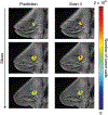
Fig. 9 ∣. Results of the 3D model predictions (over three central slices, left column) compared with the observed results at the third scan time (right column) for one example patient.

The number of tumor cells is indicated by the color overlay on each anatomical image. Notice that the model captures the correct shape of the tumor (Dice coefficient = 0.79), and while areas of higher and lower cellularity may not directly match, there are similar scales of the cellular densities between the model’s predictions and the patient’s actual tumor, resulting in Pearson and concordance correlation coefficients of 0.80 and 0.78, respectively. Comparing the summary measures of the predicted and measured tumor at scan 3 yields 13%, 17% and 4% difference in total cellularity, volume and longest axis, respectively. Informed consent was obtained from this patient.

References

Related links
1. Weis J et al. A. Cancer Res. 74, 4697–707 (2015): 10.1158/0008-5472.CAN-14-2945 - DOI - PMC - PubMed
1. Jarrett A et al. Neoplasia. 22, 820–830 (2020): 10.1016/j.neo.2020.10.011 - DOI - PMC - PubMed
1. Yankeelov TE et al. Toward a science of tumor forecasting for clinical oncology. Cancer Res. 75, 918–923 (2015). - PMC - PubMed
1. Yankeelov TE et al. Clinically relevant modeling of tumor growth and treatment response. Sci. Transl. Med 5, 187ps9 (2013). - PMC - PubMed
1. Rockne RC et al. The 2019 mathematical oncology roadmap. Phys. Biol 16, 041005 (2019). - PMC - PubMed
1. Alfonso JCL et al. The biology and mathematical modelling of glioma invasion: a review. J. R. Soc. Interface 14, 20170490 (2017). - PMC - PubMed
1. Chen X, Summers RM & Yao J Kidney tumor growth prediction by coupling reaction-diffusion and biomechanical model. IEEE Trans. Biomed. Eng 60, 169–173 (2013). - PMC - PubMed