Comparing utility functions between risky and riskless choice in rhesus monkeys

Abstract

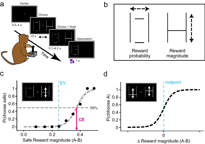
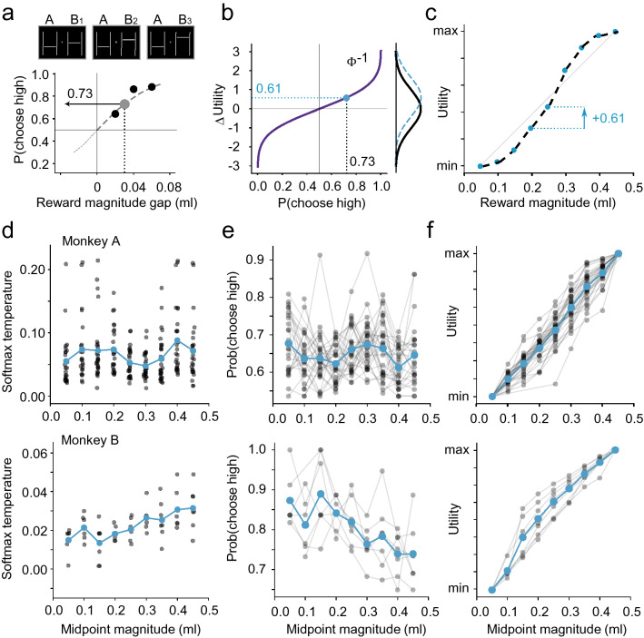
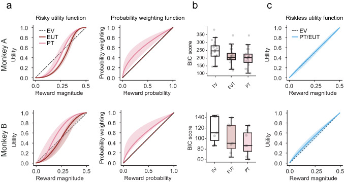
Decisions can be risky or riskless, depending on the outcomes of the choice. Expected utility theory describes risky choices as a utility maximization process: we choose the option with the highest subjective value (utility), which we compute considering both the option's value and its associated risk. According to the random utility maximization framework, riskless choices could also be based on a utility measure. Neuronal mechanisms of utility-based choice may thus be common to both risky and riskless choices. This assumption would require the existence of a utility function that accounts for both risky and riskless decisions. Here, we investigated whether the choice behavior of two macaque monkeys in risky and riskless decisions could be described by a common underlying utility function. We found that the utility functions elicited in the two choice scenarios were different from each other, even after taking into account the contribution of subjective probability weighting. Our results suggest that distinct utility representations exist for risky and riskless choices, which could reflect distinct neuronal representations of the utility quantities, or distinct brain mechanisms for risky and riskless choices. The different utility functions should be taken into account in neuronal investigations of utility-based choice.

Keywords: Decision-making; Economic choice; Gamble; Preference; Prospect theory.

Fig. 1

Experimental design and measures of risky and riskless choices. a Binary choice task. The monkeys chose one of two gambles with a left–right motion joystick. They received the blackcurrant juice reward associated with the chosen stimuli after each trial. Time, in seconds, indicate the duration of each of the task’s main events. b Schema of visual stimuli. Rewards were visually represented by horizontal lines (one or two) set between two vertical ones. The vertical position of these lines signalled the magnitude of said rewards. The width of these lines, the probability that these rewards would be realized). c Estimating certainty equivalents from risky choices. Monkeys chose between a safe reward and a risky gamble on each trial. The safe rewards alternated pseudo-randomly on every trial—they could be of any magnitude between 0 and 0.5 ml in 0.05 ml increments. Each point is a measure of choice ratio: the probability of choosing the gamble option over various safe rewards. Psychometric softmax functions (Eq. 1) were fitted to these choice ratios, then used to measure the certainty equivalents (CEs) of individual gambles (the safe magnitude for which the probability of either choice was 0.5; black arrow). The solid vertical line indicates the expected value (EV) of the gamble represented in the box. d Estimating the strength of preferences from riskless choices. Riskless safe rewards were presented against one another, the probability of choosing the higher magnitude option (A) is plotted on the y-axis as a function of the difference in magnitude between the two options presented ($\mathrm{\Delta }$ magnitude). The differences in magnitude tested were 0.02 ml, 0.04 ml, 0.06 ml, and a psychometric curve, anchored with its inflection anchored at a $\mathrm{\Delta }$ magnitude of 0, were fitted on the choice ratios measured (Eq. 2). These functions were fitted to different magnitude levels, and the temperature of each curve was linked to the strength of preferences at each of these different levels

Fig. 2

Estimating risky utilities using the fractile procedure. a Fixed utilities are mapped onto different reward magnitudes. The gambles that monkeys experienced are defined from bisections of the range of possible reward magnitudes. For each step the gambles were held fixed; safe magnitudes varied by 0.05 ml increments. b Estimation of utility using the stepwise, fractile method. In step 1, the monkeys were presented with an equivariant gamble comprised of the maximum and minimum magnitudes in the tested reward range. The CE of the gamble was estimated and assigned a utility of 50%. In step 2, two new equivariant gambles were defined from the CE elicited in step 1. The CEs of these gambles were elicited and assigned a utility of 25% and 75%. Two more gambles are defined in step 3, from the CEs elicited in step 2. Their CEs were then assigned a utility of 12.5% and 87.5%. Parametric utility functions, anchored at 0 and 1, were fitted on these utility estimates (see methods). c Utility functions estimated from choices. Data points represent daily CEs (semi-transparent) and their median values (red filled circles) tied to specific utility levels, as estimated through the fractile procedure. Both monkeys exhibit risk-seeking behaviour for low-magnitude rewards, and risk-aversion for high-magnitude ones. The data represent individual utility estimates gathered over 22 sessions for monkey A, and 7 sessions for monkey B. The red curves were obtained by fitting piecewise polynomial functions to the measured CEs (cubic splines with three knots)

Fig. 3

Estimating riskless utilities from the stochasticity in safe–safe choices. a Measuring stochasticity in choices between safe two reward options. Example visual stimuli (top) representing choices between safe rewards (A: low, B: high) resulting in different percentage of choices for the high option (bottom; black dots). This was repeated for different reward option sets, centered at different increments (midpoints). For each midpoint, the likelihoods were fitted with a softmax curve (dashed), used to estimate the probability of choosing the larger option for a gap of 0.03 ml (gray dot). b Choice ratios as differences in utility. The likelihoods that monkeys would pick the better reward were transformed using the inverse cumulative distribution function (iCDF) of a logistic distribution. The utility of different rewards took the form of equally noisy distributions centered at the true utilities. The output of iCDFs is the distance between these random utilities (i.e. the marginal utility). c From marginal utilities to utility. The cumulative sum of marginal utilities approximated a direct utility measure for each midpoint. These measurements were normalized whereby the utility of the highest midpoint was 1, and the starting midpoint had a utility of 0. d Daily strength of preference estimates. Each point represented the temperature of the softmax curve fitted on the choice ratios (blue points: average across days). The lower the temperature parameter, the steeper was the softmax curve and the more separable were the random utilities. Lower values meant higher marginal utility measurement (steeper utility function), higher ones meant lower marginal utility (flatter function). e Daily choice ratio estimates from softmax fits. Estimates from the same day are linked by grey lines. Ratios of 0.5 meant that the random utility of the two options were fully overlapping (i.e. flat utility function); choice ratios closer to 1 meant random utilities that were fully dissociated and non-overlapping. f Utility functions. Utilities estimated in single days (grey lines) and averages (blue), normalized relative to the minimum and maximum midpoint

Fig. 4

Discrete choice estimates differ between risky and riskless choices. a Utility functions in risky choice. Median parametric estimates for utility functions and probability weighting functions fitted to risky choices. Shaded area: 95% C.I. on the median of these functions. Two versions of the discrete choice model were fitted: the expected utility theory (EUT) model predicted choices solely based on reward options’ utilities (without probability weighting); the prospect theory (PT) model, predicted choices based on utilities and probability weighting. An expected value (EV) based model was included for comparison. Monkeys were risk-seeking, but where the PT model accounted for this mainly through probability weighting, the EUT model accounted for it through a more convex utility. b Comparison of risky choice models. The PT model described individual choices better than EUT and EV. Bayesian information criterions (BIC) were calculated from the log likelihoods of the daily best-fitting PT and EUT discrete choice models. c Utility functions in riskless choice. Median parametric estimates for utility functions fitted to riskless choices (shaded area: 95% C.I. on the median). The discrete choice model predicted choices from the expected utilities of rewards (no probability weighting). Utilities were mostly linear, though slightly concave

Fig. 5

Risky utilities do not predict riskless ones, and vice versa. a Median utility function estimates for risky and riskless choices. The shaded area represents the 95% C.I. on the median of these functions. For riskless choices, utility estimates were mostly linear (though slightly concave). For risky utilities, the two different versions of the discrete choice model predicted S-shaped utilities, but risky EUT utility functions were more convex than PT utility functions. b Absence of correlation for utility parameters in risky vs. riskless choices. Pearson’s correlations were run on the parameters from risky and riskless scenarios. Red squares highlight Pearson’s R for the correlation of the α and inflection parameters between risky and riskless choices. Asterisks (*) indicate significant correlations (p < 0.05)

References

1. Abdellaoui M, Barrios C, Wakker PP. Reconciling introspective utility with revealed preference: experimental arguments based on prospect theory. J Econom. 2007;138:356–378.
1. Abdellaoui M, Bleichrodt H, L’Haridon O, Paraschiv C. Is there one unifying concept of utility? An experimental comparison of utility under risk and utility over time. Manage Sci. 2013;59:2153–2169.
1. Andersen S, Harrison GW, Lau MI, Rutström EE. Eliciting risk and time preferences. Econometrica. 2008;76:583–618.
1. Andreoni J, Sprenger C. Estimating time preferences from convex budgets. Am Econ Rev. 2012;102:3333–3356.
1. Barron G, Erev I. Small feedback-based decisions and their limited correspondence to description-based decisions. J Behav Decis Mak. 2003;16:215–233.
LinkOut - more resources