A General Metric for the Similarity of Both Stochastic and Deterministic System Dynamics

Abstract

Many problems in the study of dynamical systems-including identification of effective order, detection of nonlinearity or chaos, and change detection-can be reframed in terms of assessing the similarity between dynamical systems or between a given dynamical system and a reference. We introduce a general metric of dynamical similarity that is well posed for both stochastic and deterministic systems and is informative of the aforementioned dynamical features even when only partial information about the system is available. We describe methods for estimating this metric in a range of scenarios that differ in respect to contol over the systems under study, the deterministic or stochastic nature of the underlying dynamics, and whether or not a fully informative set of variables is available. Through numerical simulation, we demonstrate the sensitivity of the proposed metric to a range of dynamical properties, its utility in mapping the dynamical properties of parameter space for a given model, and its power for detecting structural changes through time series data.

Keywords: causal discovery; change detection; chaos detection; dynamical similarity; model behavior mapping; model selection; nonlinearity.

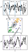
Figure 1

By fragmenting long time series, sets of appropriately selected fragments can serve as untransformed and transformed sets for estimating $$D_D$$. For two systems A and B, time series are divided into fragments of equal length (top and bottom plots), and the initial values of each segment from A and B are pooled in a common n-dimensional space (where n is the number of variables for each system) (gray arrows to center figure). For the pooled initial values, an overall mean is computed (black box, center figure) and the unit eigenvector $$\overrightarrow{v}$$ corresponding to the largest eigenvalue of the covariance matrix $$\Sigma$$ is determined (black arrow, center figure). The major and semi-major axes of the gray ellipse at the center indicates the magnitude of the first and second singular values of $$\Sigma$$. Two new means are determined by moving in opposite directions along $$\overrightarrow{v}$$ (indicated by the centers of the green and orange ellipses), and two new covariance matrices constructed by scaling the original (indicated with the major and semi-major axes of the green and orange ellipses). Finally, a predetermined number of fragments are selected for inclusion in the untransformed and transformed sets (orange +’s and green ×’s respectively) for both systems by identifying initial values (points in the plane, center figure) with the highest density according to two n-dimensional normal distributions with the newly determined means and covariance matrices.

Figure 2

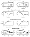
Sensitivity of $$D_D$$ to similarity of dynamical kind is demonstrated for two-species competitive Lotka–Volterra systems measured without sampling noise (a) or with normally distributed sampling noise with $$\mu =0$$ and $$\sigma =5$$) (b). Relative to a system with growth rates of $$\overrightarrow{r}=[1,2]$$ and carrying capacities, $$\overrightarrow{k}=[100,100]$$, $$D_D$$ increases as the carrying capacities $$\overrightarrow{k}$$ of the comparison system are multiplied by an increasing scaling constant such that the systems belong to diverging dynamical kinds (×), but remains approximately 0 as the growth rates $$\overrightarrow{r}$$ are scaled (+), which is a dynamical symmetry connecting systems of the same dynamical kind. When sensitivity to nonlinearity is assessed by multiplying the interaction matrix by a scale factor relative to the reference system with $$\alpha =\left[\right[1,0.5],[0.7,1\left]\right]$$, giving a linear system at a scale factor of 0, $$D_D$$ increases as the nonlinearity of the comparison system is increased (c), even in the presence of sampling noise (d). $$D_D$$ also increases between systems as their effective order diverges. For a modified Lotka–Volterra system that is second order with a scale factor of 1 and approaches first order as that scale factor tends to infinity, $$D_D$$ increases rapidly from 0 relative to a reference system with a scale factor of 1, with sampling noise (e) and without (f). $$D_D$$ also responds specifically to chaos, rising relative to a nonchaotic reference system of similar nonlinearity and order as a four-species Lotka–Volterra system passes through a chaotic transition in parameter space along the $$\beta$$ direction (defined in Equation (11)) (+), both with (g) and without (h) sampling noise. The $$l^2$$ norm (·), on the other hand, changes monotonically across the chaotic transitions.

Figure 3

Exploration of the parameter space of a four-species Lotka–Volterra model in the same $$\alpha$$-$$\beta$$ plane explored in [80] and defined in Equation (11). The absolute hue of a pixel is meaningless. However, the closer two pixels are in color, the smaller the dynamical distance $$D_D$$ between them. This color mapping is achieved by using multidimensional scaling and the distance matrix of all pairwise $$D_D$$ values to embed every point of the depicted parameter space in a three-dimensional space that is then interpreted as RGB color space.

Figure 4

(a) Dynamical distance $$D_D$$ between a stochastic, two-species Lotka–Volterra system with $$\overrightarrow{r}$$, $$\overrightarrow{k}$$, and $$\alpha$$ as in Figure 2 and one for which $$\overrightarrow{r}$$ is multiplied by the indicated scale factor (+), keeping both systems in the same dynamical kind, or for which $$\overrightarrow{k}$$ is varied (×), moving the systems into increasingly distinct dynamical kinds. (b) The same comparison as in (a) except that only the average of number of species in each system (a partial set of variables that is not SSD) is provided for computing $$D_D$$. (c) Dynamical distance between stochastic Lotka–Volterra systems of the same dynamical kind ($$\overrightarrow{r}$$, $$\overrightarrow{k}$$, and $$\alpha$$ as in (a) for one system, and $$\overrightarrow{r}$$ doubled for the other) described with an SSD (+) or non-SSD (+) set of variables, and between systems in different dynamical kinds ($$\overrightarrow{r}$$, $$\overrightarrow{k}$$, and $$\alpha$$ as in (a) for one system, and $$\overrightarrow{k}$$ doubled for the other) as a function of the parameter $$\sigma$$ which scales the Brownian term in the governing stochastic differential equation (higher $$\sigma$$ corresponds to greater stochasticity, approaching a pure Brownian process as $$\sigma \to \infty$$).

Figure 5

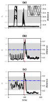
Comparison of change detection methods for a six-variable (3 phase-oscillator) Kuramoto system that transitions from uncoupled to weakly coupled over a short interval centered at 100 time units. (a) The matrix profile for each variable as a function of time (black lines); time series for all six variables are shown in the background in light gray, and over a short span of time in the inset. (b) For the same system and data as (a), the dynamical distance between two moving windows symmetrically arranged around each time is shown in black. The three standard deviation threshold for change detection is depicted as a dashed blue line while the vertical red dashed line indicates a detected change in dynamics. (c) The moving-window dynamical distance is shown (black line) for data from the same Kuramoto system but for which only one rectangular coordinate is provided from each phase oscillator (shown in light gray). The detection threshold is depicted as a dashed horizontal blue line, and the detected change event shown with a vertical dashed red line.

Figure 6

Time series from three different Kuramoto phase oscillator systems (see Equation (13)) for which each oscillator phase $${\theta }_i$$ is represented by a pair of amplitudes $$sin({\theta }_i)$$ and $$cos({\theta }_i)$$. Despite the superficial resemblance between the time series for systems A and B, the oscillators in System B are uncoupled. Systems A and C are structurally identical (every oscillator influences every other), and differ only in the set of natural frequencies, $$\omega$$.

References

1. Basseville M., Nikiforov I.V. Detection of Abrupt Changes: Theory and Application. Volume 104 Prentice Hall; Hoboken, NJ, USA: 1993.
1. Aminikhanghahi S., Cook D.J. A survey of methods for time series change point detection. Knowl. Inf. Syst. 2017;51:339–367. doi: 10.1007/s10115-016-0987-z. - DOI - PMC - PubMed
1. Yamanishi K., Takeuchi J. A Unifying Framework for Detecting Outliers and Change Points from Non-stationary Time Series Data; Proceedings of the Eighth ACM SIGKDD International Conference on Knowledge Discovery and Data Mining, KDD’02; Edmonton, AB, Canada,. 23–26 July 2002; New York, NY, USA: ACM; 2002. pp. 676–681. - DOI
1. Livina V.N., Lenton T.M. A modified method for detecting incipient bifurcations in a dynamical system. Geophys. Res. Lett. 2007;34:L03712. doi: 10.1029/2006GL028672. - DOI
1. Da C., Li F., Shen B., Yan P., Song J., Ma D. Detection of a sudden change of the field time series based on the Lorenz system. PLoS ONE. 2017;12:e0170720. doi: 10.1371/journal.pone.0170720. - DOI - PMC - PubMed
LinkOut - more resources