Application of Empirical Mode Decomposition for Decoding Perception of Faces Using Magnetoencephalography

Abstract

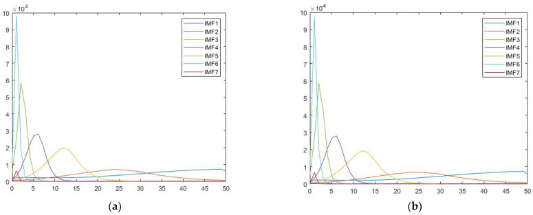
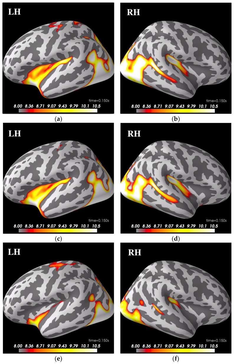
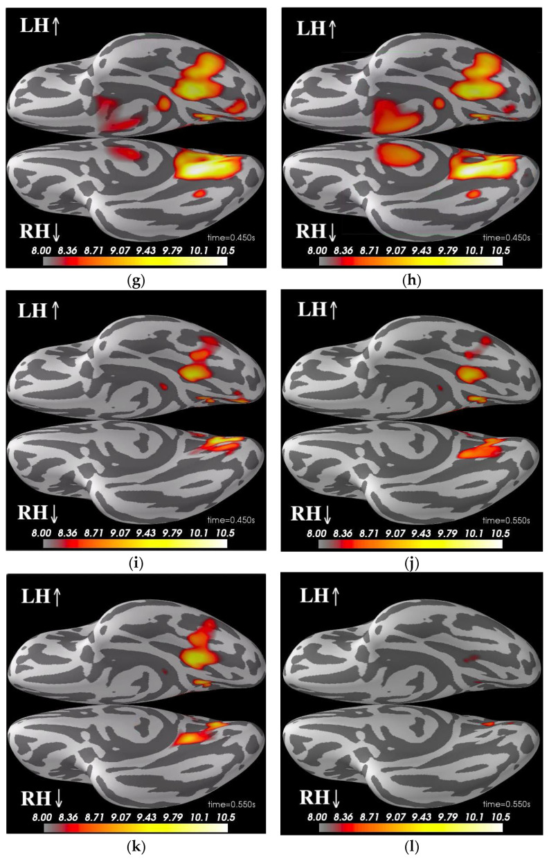
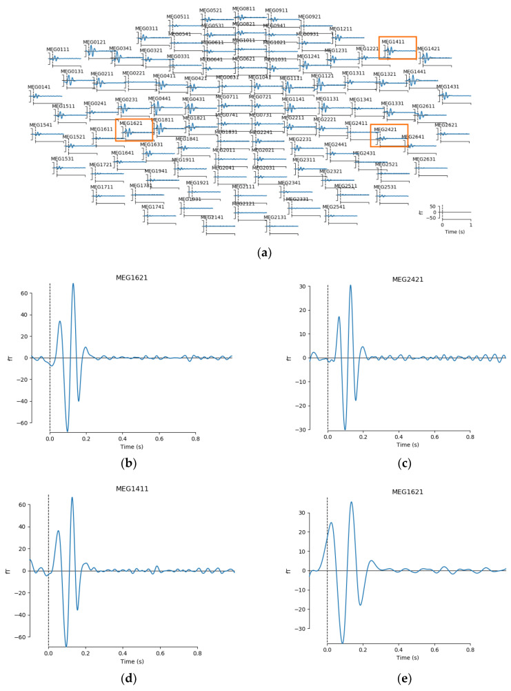
Neural decoding is useful to explore the timing and source location in which the brain encodes information. Higher classification accuracy means that an analysis is more likely to succeed in extracting useful information from noises. In this paper, we present the application of a nonlinear, nonstationary signal decomposition technique-the empirical mode decomposition (EMD), on MEG data. We discuss the fundamental concepts and importance of nonlinear methods when it comes to analyzing brainwave signals and demonstrate the procedure on a set of open-source MEG facial recognition task dataset. The improved clarity of data allowed further decoding analysis to capture distinguishing features between conditions that were formerly over-looked in the existing literature, while raising interesting questions concerning hemispheric dominance to the encoding process of facial and identity information.

Keywords: empirical mode decomposition (EMD); face perception; magnetoencephalography (MEG); neural decoding.

Figure 1

This figure shows the step-by-step data processing procedures along with all the analyses that we performed.

Figure 2

This figure shows the Hilbert spectra for (a) famous, (b) scrambled face conditions for participant 001 in the dataset. The x-axis is frequency (Hz), and the y-axis is energy (a.u.).

Figure 3

This figure shows dSPM source localization, the significant activities demonstrated here are: (a) famous condition IMF4 at 150 ms in left hemisphere (LH); (b) famous condition IMF4 at 150 ms in right hemisphere (RH); (c) unfamiliar condition IMF4 at 150 ms in LH; (d) unfamiliar condition IMF4 at 150 ms in RH; (e) scrambled condition IMF4 at 150 ms in LH; (f) scrambled condition IMF4 at 150 ms in RH; (g) famous condition IMF5 at 450 ms in ventral view; (h) unfamiliar condition IMF5 at 450 ms in ventral view; (i) scrambled condition IMF5 at 450 ms in ventral view; (j) famous condition IMF6 at 550 ms in ventral view; (k) unfamiliar condition IMF6 at 550 ms in ventral view; (l) scrambled condition IMF6 at 550 ms in ventral view.

Figure 3

This figure shows dSPM source localization, the significant activities demonstrated here are: (a) famous condition IMF4 at 150 ms in left hemisphere (LH); (b) famous condition IMF4 at 150 ms in right hemisphere (RH); (c) unfamiliar condition IMF4 at 150 ms in LH; (d) unfamiliar condition IMF4 at 150 ms in RH; (e) scrambled condition IMF4 at 150 ms in LH; (f) scrambled condition IMF4 at 150 ms in RH; (g) famous condition IMF5 at 450 ms in ventral view; (h) unfamiliar condition IMF5 at 450 ms in ventral view; (i) scrambled condition IMF5 at 450 ms in ventral view; (j) famous condition IMF6 at 550 ms in ventral view; (k) unfamiliar condition IMF6 at 550 ms in ventral view; (l) scrambled condition IMF6 at 550 ms in ventral view.

Figure 4

This figure shows MEG activity patterns from sensor level analysis. Here we see: (a) location of the selected channels; (b) IMF5 activities at channel 1621 (left supramarginal); (c) IMF5 activities at channel 2421 (right supramarginal); (d) IMF5 activities at channel 1411 (inferior frontal); (e) IMF6 activities at channel 1621; (f) IMF6 activities at channel 2421; (g) IMF5 activities at channel 1411.

Figure 4

This figure shows MEG activity patterns from sensor level analysis. Here we see: (a) location of the selected channels; (b) IMF5 activities at channel 1621 (left supramarginal); (c) IMF5 activities at channel 2421 (right supramarginal); (d) IMF5 activities at channel 1411 (inferior frontal); (e) IMF6 activities at channel 1621; (f) IMF6 activities at channel 2421; (g) IMF5 activities at channel 1411.

Figure 5

This figure shows dSPM source localization of the simulated data. IMF5 appears to capture higher level of activities than IMF6. (a) IMF5 at 130 ms in the RH; (b) IMF5 at 130 ms in the LH; (c) IMF6 at 130 ms in the RH; (d) IMF6 at 130 ms in the LH.

Figure 6

This section shows the statistical results of significant pattern differences between conditions. The x-axis is time, while the y-axis is t score. (a) famous and scrambled pairing (FS), IMF4; (b) unfamiliar and scrambled pairing (US), IMF4; (c) famous and unfamiliar pairing (FU), IMF4; (d) famous and scrambled pairing (FS), IMF5; (e) unfamiliar and scrambled pairing (US), IMF5; (f) famous and unfamiliar pairing (FU), IMF5; (g) famous and scrambled pairing (FS), IMF6; (h) unfamiliar and scrambled pairing (US), IMF6; (i) famous and unfamiliar pairing (FU), IMF6.

Figure 6

This section shows the statistical results of significant pattern differences between conditions. The x-axis is time, while the y-axis is t score. (a) famous and scrambled pairing (FS), IMF4; (b) unfamiliar and scrambled pairing (US), IMF4; (c) famous and unfamiliar pairing (FU), IMF4; (d) famous and scrambled pairing (FS), IMF5; (e) unfamiliar and scrambled pairing (US), IMF5; (f) famous and unfamiliar pairing (FU), IMF5; (g) famous and scrambled pairing (FS), IMF6; (h) unfamiliar and scrambled pairing (US), IMF6; (i) famous and unfamiliar pairing (FU), IMF6.

Figure 7

Here we compiled the activity pattern differences in the LH and RH. The x-axis is time, and the y-axis is t score. The red area is where the t-statistic level in the LH is larger than the RH. (a) FU pairing activity differences on IMF6 in the fusiform area; (b) FU pairing activity differences on IMF6 in the inferior temporal area; (c) FS pairing activity differences on IMF5 in the frontal area; (d) FS pairing activity differences on IMF6 in the frontal area; (e)FS pairing activity differences on IMF6 in the inferior temporal area; (f) FS pairing activity differences on IMF6 in the temporal pole.

References

1. Klonowski W. Everything You Wanted to Ask about EEG but Were Afraid to Get the Right Answer. Nonlinear Biomed. Phys. 2009;3:2. doi: 10.1186/1753-4631-3-2. - DOI - PMC - PubMed
1. Stallone A., Cicone A., Materassi M. New Insights and Best Practices for the Successful Use of Empirical Mode Decomposition, Iterative Filtering and Derived Algorithms. Sci. Rep. 2020;10:15161. doi: 10.1038/s41598-020-72193-2. - DOI - PMC - PubMed
1. Huang N.E., Shen Z., Long S.R., Wu M.C., Shih H.H., Zheng Q., Yen N.-C., Tung C.C., Liu H.H. The Empirical Mode Decomposition and the Hilbert Spectrum for Nonlinear and Non-Stationary Time Series Analysis. Proc. R. Soc. London. Ser. A Math. Phys. Eng. Sci. 1998;454:903–995. doi: 10.1098/rspa.1998.0193. - DOI
1. Nguyen K.T., Liang W.-K., Lee V., Chang W.-S., Muggleton N.G., Yeh J.-R., Huang N.E., Juan C.-H. Unraveling Nonlinear Electrophysiologic Processes in the Human Visual System with Full Dimension Spectral Analysis. Sci. Rep. 2019;9:16919. doi: 10.1038/s41598-019-53286-z. - DOI - PMC - PubMed
1. Wakeman D.G., Henson R.N. A Multi-Subject, Multi-Modal Human Neuroimaging Dataset. Sci. Data. 2015;2:150001. doi: 10.1038/sdata.2015.1. - DOI - PMC - PubMed