A more accurate method for colocalisation analysis allowing for multiple causal variants

Abstract

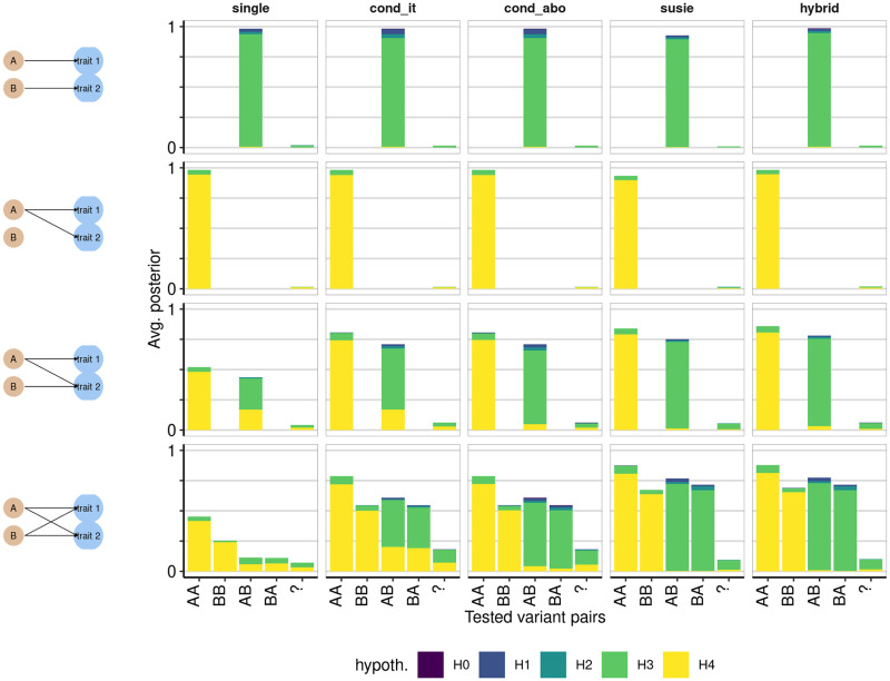
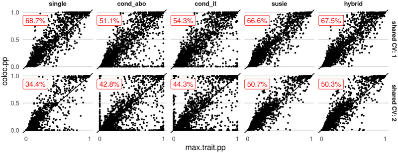
In genome-wide association studies (GWAS) it is now common to search for, and find, multiple causal variants located in close proximity. It has also become standard to ask whether different traits share the same causal variants, but one of the popular methods to answer this question, coloc, makes the simplifying assumption that only a single causal variant exists for any given trait in any genomic region. Here, we examine the potential of the recently proposed Sum of Single Effects (SuSiE) regression framework, which can be used for fine-mapping genetic signals, for use with coloc. SuSiE is a novel approach that allows evidence for association at multiple causal variants to be evaluated simultaneously, whilst separating the statistical support for each variant conditional on the causal signal being considered. We show this results in more accurate coloc inference than other proposals to adapt coloc for multiple causal variants based on conditioning. We therefore recommend that coloc be used in combination with SuSiE to optimise accuracy of colocalisation analyses when multiple causal variants exist.

Fig 1. Average posterior probability distributions in simulated data.

The four classes of simulated datasets are shown in four rows, with the scenario indicated in the left hand column. For example, the top row shows a scenario where traits 1 and 2 have distinct causal variants A and B. Columns indicate the different analysis methods, with susie indicating SuSiE, cond_it indicating that coloc-conditioning was run in iterative mode, and cond_abo indicating it was run in “all but one” mode. For each simulation, the number of tests performed is at most 1 for “single”, or equal to the product of the number of signals detected for the other methods. For each test, we estimated which pair of variants were being tested according to the LD between the variant with highest fine-mapping posterior probability of causality for each trait and the true causal variants A and B. If r² > 0.5 between the fine-mapped variant and true causal variant A, and r² with A was higher than r² with B, we labeled the test variant A, and vice versa for B. Where at least one test variant could not be unambigously assigned, we labelled the pair “?”. The total height of each bar represents the proportion of comparisons that were run for that variant pair, out of the number of simulations run, and typically does not reach 1 because there is not always power to perform all possible tests. Note that because we do not limit the number of tests, the height of the bar has the potential to exceed 1, but did not do so in practice. The shaded proportion of each bar corresponds to the average posterior for the indicated hypothesis, defined as the ratio of the sum of posterior probabilities for that hypothesis to the number of simulations performed. Recall that H₀ indicates no associated variants for either trait, H₁ and H₂ a single causal variant for traits 1 and 2 respectively, H₃ and H₄ that both traits are associated with either distinct or shared causal variants, respectively. Each simulated region contains 1000 SNPs.

Fig 2. Distribution of maximum -log10 p values for simulated datasets where coloc-SuSiE could find at least one credible set for each trait, or could not.

Each dataset was summarised by its maximum -log10 p value, and the pair of datasets by the minimum of these. A dashed line shows the conventional GWAS significance threshold of 5 × 10⁻⁸. This shows that when coloc-SuSiE does not produce any results it is generally in cases of lower power.

Fig 3. Example where the conditional coloc approach, run in iterative mode, finds misleading results.

a and b show the “observed” data (simulated from 1000 SNPs with MAF > 0.01) as -log₁₀ p values for traits 1 and 2 respectively. Trait 1 has one causal variant, A, and trait 2 has two, A and B. Conditioning identifies a second independent signal for trait 2, and the results of conditioning on the strongest signal is shown in c. Coloc comparisons are based on (a, b) and (a, c) and both find the posterior probability (PP) of the shared causal variant hypothesis H₄ is > 0.8. SuSiE analysis of the same data finds one credible set in trait 1, and log₁₀ Bayes factors (BF) for this are shown in d. It finds two credible sets for trait 2, and the log₁₀ BF for these are shown in e and f. Coloc comparisons are based on (d, e) and (d, f) and find PP of H₄ of > 0.9 and < 10⁻⁴ respectively. Blue and green points are used to highlight SNPs in LD with (r² > 0.8) the true causal variants A and B respectively. The data underlying this figure are available in S1 Data.

Fig 4. Fine mapping posterior probabilities at causal variants in single trait and coloc analysis, amongst datasets with high probability of colocalisation (P(H₄|Data) > 0.9) according to the method shown.

Each point represents one causal variant in a dataset; its x location shows its maximum fine mapping posterior probability (PP) in either single trait, its y location shows its PP after coloc. Results are divided by rows into those from datasets with 1 (top) or 2 (bottom) causal variants, and by columns according to method. The text in red shows the percent of datasets which led to an increase in PP at causal variants after coloc analysis.

References

1. Giambartolomei C, Vukcevic D, Schadt EE, Franke L, Hingorani AD, Wallace C, et al. Bayesian Test for Colocalisation between Pairs of Genetic Association Studies Using Summary Statistics. PLOS Genetics. 2014. May;10(5):e1004383. Available from: http://journals.plos.org/plosgenetics/article?id=10.1371/journal.pgen.10.... - PMC - PubMed
1. Wakefield J. Bayes Factors for Genome-Wide Association Studies: Comparison with P -Values. Genet Epidemiol. 2009. Jan;33(1):79–86. Available from: 10.1002/gepi.20359. - DOI - PubMed
1. Wallace C. Eliciting Priors and Relaxing the Single Causal Variant Assumption in Colocalisation Analyses. PLOS Genetics. 2020. Apr;16(4):e1008720. Available from: https://journals.plos.org/plosgenetics/article?id=10.1371/journal.pgen.1.... - PMC - PubMed
1. The Wellcome Trust Case Control Consortium, Maller JB, McVean G, Byrnes J, Vukcevic D, Palin K, et al. Bayesian Refinement of Association Signals for 14 Loci in 3 Common Diseases. Nat Genet. 2012. Oct;44(12):1294–1301. Available from: 10.1038/ng.2435. - DOI - PMC - PubMed
1. Hormozdiari F, van de Bunt M, Segre AV, Li X, Joo JWJ, Bilow M, et al. Colocalization of GWAS and eQTL Signals Detects Target Genes. Am J Hum Genet. 2016;99(6):1245–1260. Available from: 10.1016/j.ajhg.2016.10.003. - DOI - PMC - PubMed
Publication types