A random-walk-based epidemiological model

Abstract

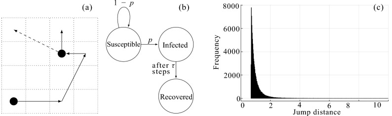
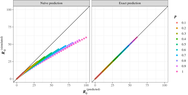
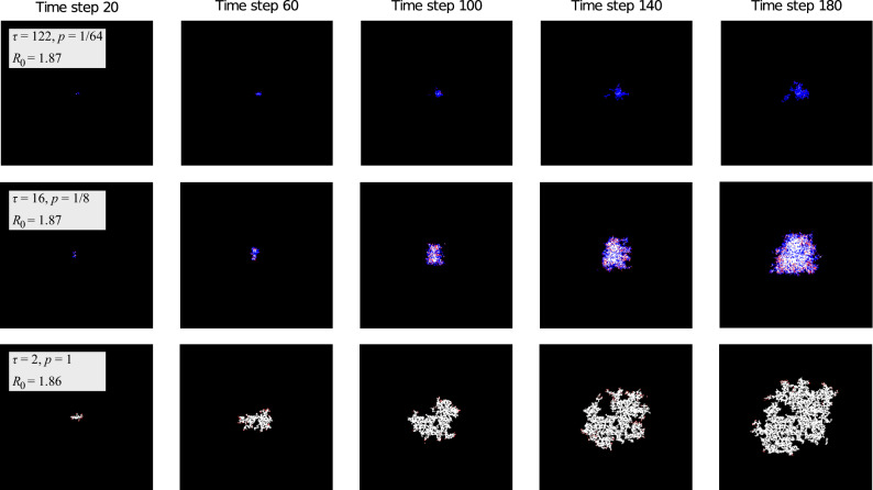
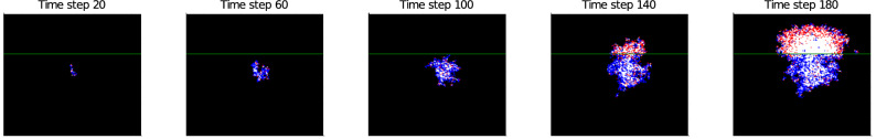
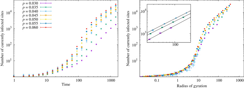
Random walkers on a two-dimensional square lattice are used to explore the spatio-temporal growth of an epidemic. We have found that a simple random-walk system generates non-trivial dynamics compared with traditional well-mixed models. Phase diagrams characterizing the long-term behaviors of the epidemics are calculated numerically. The functional dependence of the basic reproductive number [Formula: see text] on the model's defining parameters reveals the role of spatial fluctuations and leads to a novel expression for [Formula: see text]. Special attention is given to simulations of inter-regional transmission of the contagion. The scaling of the epidemic with respect to space and time scales is studied in detail in the critical region, which is shown to be compatible with the directed-percolation universality class.

Figure 1

The model. (a) A walker (solid line) at some step infects a susceptible site, which generates another walker (dashed line). (b) The walker state diagram for each step, where p and $1-p$ transitions are triggered by infectious-susceptible interactions. (c) Histogram of jump distances of infective agents for 100,000 realizations.

Figure 2

The prediction for $R_0$ and simulation data. Left panel: actual $R_0^{\text{(simulated)}}$ against the naïve prediction of Eq. (1), $R_0^{\text{(predicted)}}=p\tau$. Right panel: $R_0^{\text{(simulated)}}$ against the prediction of Eq. (4). The straight line is $R_0^{(\text{simulated})}=R_0^{(\text{predicted})}$. Each dot corresponds to a combination of p and $\tau$ (the values of p are color coded, $\tau$ is between 1 and 100).

Figure 3

Progression of the outbreak. Red sites are infective agents, white are removed and black are susceptible. Blue sites are not technically part of the SIR categories but represent susceptible sites which have been previously visited (but not infected). This fourth color brings attention to the pockets of susceptibles left in the wake of the infection. Note that the model exhibits very different behavior for combinations of $\tau$ and p with almost identical $R_0$, demonstrating that $R_0$ is not always an accurate characterization of the overall behavior of an outbreak. For example, the outbreak in the bottom row grew much more rapidly in the earlier time steps, but by the final time step, the outbreak in the middle row had a much larger population of active infective agents. Nonetheless, the cumulative number of infections is much higher in the former.The outbreak shown in the top row is clearly of much smaller magnitude despite having the same $R_0$. The boxes are $300\times 300$ sites.

Figure 4

Phase diagram in log-log scale, including iso-$R_0$ lines. The heatmap scale shows the phase variable of Eq. (6), namely, the fraction of realizations where the outbreak dies out. While a continuous red-orange color scale is used to plot the phase variable, the phase diagram appears as essentially a binary plot of two colors. This behavior reflects the sharp transition.

Figure 5

Simulation of an outbreak spanning two regions with distinct p values. The border between the two regions is located at the green $y=100$ line and the infection originates at the center of the grid. Once crossing the boundary to the upper region, the infection explodes. For $y\le 100$, $p=0.1$ and for $y>100$, $p=0.3$. This illustrates a stark example of the effects of an infection re-igniting upon crossing a regional border. The boxes are $150\times 150$ sites.

Figure 6

Spatial growth of the outbreak with time. (a) Total number of removed sites (total epidemic size) as a function of time in a log-log scale. (b) Same quantity as a function of the radius of gyration. The inset shows a closeup to appreciate the power-law fit. (c) Normalized spatial autocorrelation of the set of removed sites, $\rho$ in Eq. (9), for $p=0.05$. (d) Spatial autocorrelation in semi-log scale as a function of $r/{\mathcal{R}}_{\text{g}}$. Again, using ${\mathcal{R}}_{\text{g}}$ as scaling variable leads to an enveloping curve.

Figure 7

Growth of the number of currently infected sites, against time (left) and against the radius of gyration of the set (right). In this case the curves for different p do not collapse, but the curves approach a power law $I\propto {\mathcal{R}}_{\text{g},I}^{d_{\cap }}$ with $d_{\cap }=1.18(5)$, see Eq. (12). This exponent is compatible with the directed-percolation universality class. The inset shows a closeup of the fits for $p=0.03,0.035,0.04$.

References

1. Allen LJS. A primer on stochastic epidemic models: Formulation, numerical simulation, and analysis. Infect. Dis. Model. 2017;2:128–142. doi: 10.1016/j.idm.2017.03.001. - DOI - PMC - PubMed
1. Hethcote HW. The mathematics of infectious diseases. SIAM Rev. 2000;42:599–653. doi: 10.1137/S0036144500371907. - DOI
1. Grijalva CG, et al. Transmission of SARS-COV-2 infections in households—Tennessee and Wisconsin, April–September 2020. Morb. Mortal. Wkly. Rep. 2020 doi: 10.15585/mmwr.mm6944e1. - DOI - PMC - PubMed
1. Huber G, et al. A minimal model for household effects in epidemics. Phys. Biol. 2020;17:065010. doi: 10.1088/1478-3975/abb209. - DOI - PubMed
1. Bittihn P, Hupe L, Isensee J, Golestanian R. Local measures enable COVID-19 containment with fewer restrictions due to cooperative effects. EClin. Med. 2021;32:100718. doi: 10.1016/j.eclinm.2020.100718. - DOI - PMC - PubMed
Publication types