. 2022 Aug;54(4):1663-1687.
doi: 10.3758/s13428-021-01703-5. Epub 2021 Sep 29.

MouseView.js: Reliable and valid attention tracking in web-based experiments using a cursor-directed aperture

Affiliations

MouseView.js: Reliable and valid attention tracking in web-based experiments using a cursor-directed aperture

Alexander L Anwyl-Irvine et al. Behav Res Methods. 2022 Aug.

Abstract

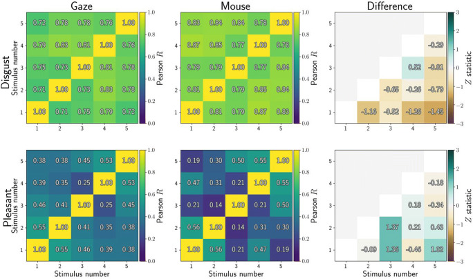
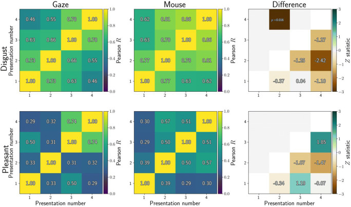
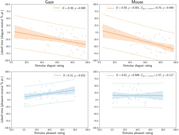
Psychological research is increasingly moving online, where web-based studies allow for data collection at scale. Behavioural researchers are well supported by existing tools for participant recruitment, and for building and running experiments with decent timing. However, not all techniques are portable to the Internet: While eye tracking works in tightly controlled lab conditions, webcam-based eye tracking suffers from high attrition and poorer quality due to basic limitations like webcam availability, poor image quality, and reflections on glasses and the cornea. Here we present MouseView.js, an alternative to eye tracking that can be employed in web-based research. Inspired by the visual system, MouseView.js blurs the display to mimic peripheral vision, but allows participants to move a sharp aperture that is roughly the size of the fovea. Like eye gaze, the aperture can be directed to fixate on stimuli of interest. We validated MouseView.js in an online replication (N = 165) of an established free viewing task (N = 83 existing eye-tracking datasets), and in an in-lab direct comparison with eye tracking in the same participants (N = 50). Mouseview.js proved as reliable as gaze, and produced the same pattern of dwell time results. In addition, dwell time differences from MouseView.js and from eye tracking correlated highly, and related to self-report measures in similar ways. The tool is open-source, implemented in JavaScript, and usable as a standalone library, or within Gorilla, jsPsych, and PsychoJS. In sum, MouseView.js is a freely available instrument for attention-tracking that is both reliable and valid, and that can replace eye tracking in certain web-based psychological experiments.

Keywords: Attention; JavaScript; cyberpsychology; eye tracking; online experiments; open-source.


Conflict of interest statement

All authors would benefit from the publication of this manuscript in the sense that it would increase their competitiveness for academic jobs and grants. Author Anwyl-Irvine was previously under part-time employment at Cauldron. This company maintains the Gorilla experiment builder, and can potentially stand to gain from the open-source software presented in this manuscript. It should be noted that this benefit exists for every company that operates within the same industry, as the software presented in this manuscript is released under the MIT license, and therefore freely available for commercial use, modification, and distribution.

Figures

Fig. 1
Fig. 1
Screenshots of different MouseView.js configurations. a Solid black overlay with Gaussian Edge SD of 5 pixels (overlayColour=’black’, overlayAlpha=1, overlayGaussian=0, apertureGauss=5). b Gaussian overlay and Gaussian aperture edge with SD of 50 pixels (overlayColour=’black’, overlayAlpha=0.8, overlayGaussian=20, apertureGauss=50). c Gaussian overlay with solid aperture edge (overlayColour=’black’, overlayAlpha=0.8, overlayGaussian=20, apertureGauss=0). d No Gaussian blur but overlay with 0.9 alpha opacity (overlayColour=’black’, overlayAlpha=0.9, overlayGaussian=0, apertureGauss=10). e Gaussian blurred overlay with 0.0 opacity (overlayColour=’black’, overlayAlpha=0, overlayGaussian=20, apertureGauss=10). f Pink overlay (overlayColour=’#FF69B4’, overlayAlpha=0.8, overlayGaussian=0, apertureGauss=10)
Fig. 2
Fig. 2
Correlations between affective-neutral dwell time differences for all stimuli (averaged across all four presentations). Higher correlations indicate that participants showed similar dwell time differences between stimuli. Included here are five disgust stimuli (top row) and five pleasant stimuli (bottom row). Dwell times were computed from eye tracking (left column) or MouseView.js (middle column), and the difference between them is reported in the right column
Fig. 3
Fig. 3
Correlations between affective-neutral dwell time differences for all repetitions of the same stimuli (averaged across all five stimuli within each condition). Higher correlations indicate that participants showed similar dwell time differences between repetitions. Included here are four repetitions of five disgust stimuli (top row) and five pleasant stimuli (bottom row). Dwell times were computed from eye tracking (left column) or MouseView.js (middle column), and the difference between them is reported in the right column
Fig. 4
Fig. 4
Gaze dwell time difference (in percentage points) between affective and neutral stimuli as obtained in an eye-tracking task. Positive values indicate participants spent more time looking at the affective (disgust or pleasant) stimulus than the control stimulus; negative values indicate the opposite. In the top row, solid lines indicate averages and shading the within-participant 95% confidence interval. In the bottom row, t values from one-samplet tests of the dwell difference against 0 are reported, but only for those tests where p < 0.05 (uncorrected)
Fig. 5
Fig. 5
Mouse dwell time difference (in percentage points) between affective and neutral stimuli as obtained in a MouseView.js task. Positive values indicate participants spent more time looking at the affective (disgust or pleasant) stimulus than the control stimulus; negative values indicate the opposite. In the top row, solid lines indicate averages and shading the within-participant 95% confidence interval. The sharp return to 0 at the end of the trial duration is an artefact of mouse recording cutting out slightly too early. In the bottom row, t values from one-samplet tests of the dwell difference against 0 are reported, but only for those tests where p < 0.05 (uncorrected)
Fig. 6
Fig. 6
Quantification of the difference between gaze dwell time differences (eye tracking, Fig. 4) and mouse dwell times (MouseView.js, Fig. 5). Positive values indicate higher avoidance of the affective stimulus (compared to the neutral stimulus) in MouseView.js compared to eye tracking, and negative values indicate higher avoidance of the affective stimulus in eye tracking. In the top panels, the dashed line indicates the average, and the shaded area the 95% confidence interval (based on between-participant pooled standard error of the mean, computed through Satterthwaite approximation). In the bottom row, Bayes factors quantify evidence for the alternative hypothesis (gaze and mouse are different) or the null hypothesis (gaze and mouse result in similar dwell-time differences). A log(BF10) of 1.1 corresponds with a BF10 of 3 (evidence for alternative), whereas a log(BF10) of – 1.1 corresponds with a BF01 of 3 (evidence for null)
Fig. 7
Fig. 7
Correlation between the average self-reported disgust (top row) or pleasantness rating (bottom row) and the affective-neutral difference in dwell time. Ratings were averaged across all stimuli within each condition, and dwell times across all stimuli and stimulus presentations within each condition. The reported Z and uncorrected p values quantify the difference between dwell times obtained with eye tracking (left column) and MouseView.js (right column). Solid lines indicate the linear regression line, and the shaded area the error of the estimate
Fig. 8
Fig. 8
Heatmaps (two-dimensional histogram of resampled (x,y) coordinates) for all five disgust stimuli. The top row quantifies samples obtained from an eye-tracking experiment and the bottom row from a MouseView.js experiment. Brighter colours indicate more observations falling within that area. Note that, in reality, stimulus position was pseudo-random, but that samples were flipped where necessary so that the affective stimulus appeared on the left. Stimulus images are strongly blurred to obscure their content, as their usage license prevents publication
Fig. 9
Fig. 9
Heatmaps (two-dimensional histogram of resampled (x,y) coordinates) for all five pleasant stimuli. The top row quantifies samples obtained from an eye-tracking experiment and the bottom row from a MouseView.js experiment. Brighter colours indicate more observations falling within that area. Note that, in reality, stimulus position was pseudo-random, but that samples were flipped where necessary so that the affective stimulus appeared on the left. Stimulus images are strongly blurred to obscure their content, as their usage license prevents publication
Fig. 10
Fig. 10
Three-dimensional scanpaths (horizontal and vertical coordinate, and time) reduced into two dimensions using multi-dimensional scaling (MDS). Each dot represents a single scanpath (i.e. a single trial). The top row shows scanpaths for disgust and neutral stimuli and the bottom row from the pleasant and neutral stimuli. The left column shows gaze (from eye tracking) scanpaths in colour and mouse (from MouseView.js) in grey; whereas the right column shows the opposite
Fig. 11
Fig. 11
Three-dimensional scanpaths (horizontal and vertical coordinate, and time) reduced into two dimensions using uniform manifold approximation and projection (UMAP). Each dot represents a single scanpath (i.e. a single trial). The top row shows scanpaths for disgust and neutral stimuli and the bottom row from the pleasant and neutral stimuli. The left column shows gaze (from eye tracking) scanpaths in colour and mouse (from MouseView.js) in grey; whereas the right column shows the opposite
Fig. 12
Fig. 12
Correlations between affective-neutral dwell time differences for all stimuli (averaged across all four presentations). Higher correlations indicate that participants showed similar dwell time differences between stimuli. Included here are five disgust stimuli (top row) and five pleasant stimuli (bottom row). Dwell times were computed from eye tracking (left column) or MouseView.js (middle column), and the difference between them is reported in the right column
Fig. 13
Fig. 13
Correlations between affective-neutral dwell time differences for all stimuli (averaged across all four presentations). Higher correlations indicate that participants showed similar dwell time differences between stimuli. Included here are five disgust stimuli (top row) and five pleasant stimuli (bottom row). Dwell times were computed from eye tracking (left column) or MouseView.js (middle column), and the difference between them is reported in the right column
Fig. 14
Fig. 14
Gaze dwell time difference (in percentage points) between affective and neutral stimuli as obtained in an eye-tracking task. Positive values indicate participants spent more time looking at the affective (disgust or pleasant) stimulus than the neutral stimulus and negative values indicate the opposite. In the top row, solid lines indicate averages, and shading the within-participant 95% confidence interval. The bottom row shows t values from one-samplet tests of the dwell-difference compared to 0, for those tests where p < 0.05 (uncorrected). Positive t values (pink) indicate higher dwell time for the affective stimulus (approach), and negative t values (green) indicate higher dwell time for the neutral stimulus (avoidance)
Fig. 15.
Fig. 15.
Mouse dwell time difference (in percentage points) between affective and neutral stimuli as obtained in a web-based MouseView.js task. Positive values indicate participants spent more time looking at the affective (disgust or pleasant) stimulus than the neutral stimulus and negative values indicate the opposite. In the top row, solid lines indicate averages, and shading the within-participant 95% confidence interval. The sharp return to 0 at the end of the trial duration is an artefact of mouse recording cutting out slightly too early. The bottom row shows t values from one-samplet tests of the dwell-difference compared to 0, for those tests where p < 0.05 (uncorrected). Positive t values (pink) indicate higher dwell time for the affective stimulus (approach), and negative t values (green) indicate higher dwell time for the neutral stimulus (avoidance)
Fig. 16
Fig. 16
Quantification of the difference between gaze dwell time differences (eye tracking, Fig. 14) and mouse dwell time differences (MouseView.js, Fig. 15). Positive values indicate higher avoidance of the affective stimulus (compared to the neutral stimulus) in MouseView.js compared to eye tracking and negative values indicate higher avoidance of the affective stimulus in eye tracking. In the top panels, dashed lines indicate the average and the shaded area the 95% within-participant confidence interval. In the bottom panels, Bayes factors quantify evidence for the alternative hypothesis (gaze and mouse are different) or the null hypothesis (gaze and mouse are not different); each quantified as a linear mixed model with participant as random effect, and the alternative model with method (gaze/mouse) as fixed effect. A log(BF10) of 1.1 corresponds with a BF10 of 3 (evidence for the alternative), whereas a log(BF10) of – 1.1 corresponds with a BF01 of 3 (evidence for the null)
Fig. 17
Fig. 17
Quantification of the relationship between eye tracking and MouseView.js dwell time differences between disgust (red) or pleasant (blue) and neutral stimuli. The top panels show the regression line, with the error of the estimate shaded, and individuals plotted as dots. The bottom panels show the Pearson correlation between gaze and mouse per time bin (solid line) and its standard error (shaded area). Values that fall within the grey area are not statistically significant, with the dotted lines indicating the critical values for R where p = 0.05
Fig. 18
Fig. 18
Correlation between the average self-reported disgust (red, top row) or pleasantness rating (blue, bottom row) and the affective-neutral difference in dwell time. Ratings were averaged across all stimuli within each condition, and dwell times across all stimuli and stimulus presentations within each condition. The reported Z and (uncorrected)p values quantify the difference between the correlations for eye tracking (left column) and MouseView.js (right column). Solid lines indicate the linear regression line and the shaded area the error of the estimate. Dots represent individual participants

References

    1. Ang Y-S, Manohar S, Plant O, Kienast A, Le Heron C, Muhammed K, Hu M, Husain M. Dopamine modulates option generation for behavior. Current Biology. 2018;28(10):1561–1569.e3. doi: 10.1016/j.cub.2018.03.069. - DOI - PMC - PubMed
    1. Anwyl-Irvine, A. L., Dalmaijer, E. S., Hodges, N., & Evershed, J. K. (2020a). Realistic precision and accuracy of online experiment platforms, web browsers, and devices. Behavior Research Methods. 10.3758/s13428-020-01501-5 - PMC - PubMed
    1. Anwyl-Irvine AL, Massonnié J, Flitton A, Kirkham N, Evershed JK. Gorilla in our midst: An online behavioral experiment builder. Behavior Research Methods. 2020;52(1):388–407. doi: 10.3758/s13428-019-01237-x. - DOI - PMC - PubMed
    1. Armstrong T, Olatunji BO. Eye tracking of attention in the affective disorders: A meta-analytic review and synthesis. Clinical Psychology Review. 2012;32(8):704–723. doi: 10.1016/j.cpr.2012.09.004. - DOI - PMC - PubMed
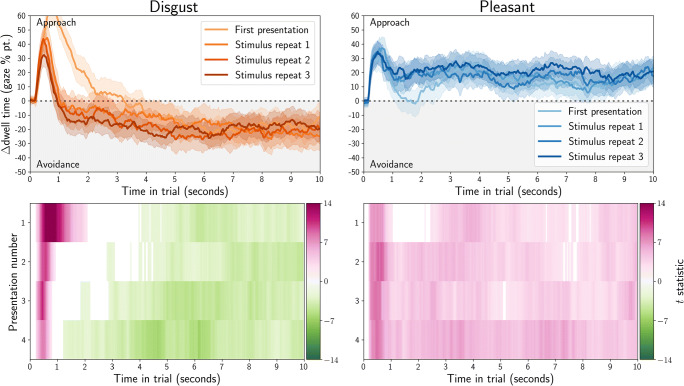
    1. Armstrong, T., Stewart, J. G., Dalmaijer, E. S., Rowe, M., Danielson, S., Engel, M., Bailey, B., & Morris, M. (2020). I’ve seen enough! Prolonged and repeated exposure to disgusting stimuli increases oculomotor avoidance. Emotion. 10.1037/emo0000919 - PubMed

Publication types

LinkOut - more resources