Impulsive Fire Disturbance in a Savanna Model: Tree-Grass Coexistence States, Multiple Stable System States, and Resilience

Abstract

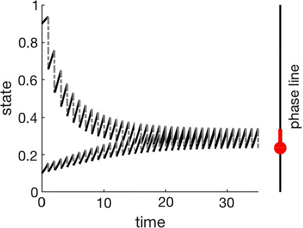
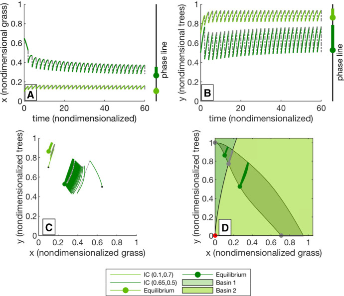
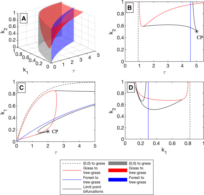
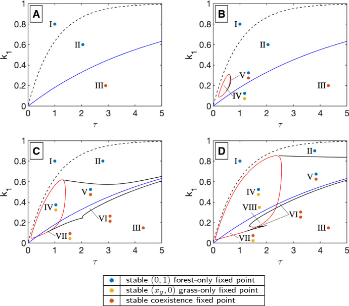
Savanna ecosystems are shaped by the frequency and intensity of regular fires. We model savannas via an ordinary differential equation (ODE) encoding a one-sided inhibitory Lotka-Volterra interaction between trees and grass. By applying fire as a discrete disturbance, we create an impulsive dynamical system that allows us to identify the impact of variation in fire frequency and intensity. The model exhibits three different bistability regimes: between savanna and grassland; two savanna states; and savanna and woodland. The impulsive model reveals rich bifurcation structures in response to changes in fire intensity and frequency-structures that are largely invisible to analogous ODE models with continuous fire. In addition, by using the amount of grass as an example of a socially valued function of the system state, we examine the resilience of the social value to different disturbance regimes. We find that large transitions ("tipping") in the valued quantity can be triggered by small changes in disturbance regime.

Keywords: Bistability; Impulsive differential equations; Resilience; Savanna; Tipping points; Transient dynamics.

Fig. 1

The plot shows two time series, with different initial conditions, for an impulsive differential equation. In this example, the state variable flows according to $\dot{x}=\frac{1}{2}x(1-x)$ for a period of one time unit. The state variable then experiences an impulse (kick) proportional to its state at the end of the flow period, $\mathrm{\Delta }x(t_n)=x(t_n^{+})-x(t_n^{-})=-0.3x(t_n^{-})$ with $t_n=n$. The two time series are converging to an asymptotically stable periodic solution of the impulsive system, which is shown in red on the phase line. The red dot denotes the fixed point of the associated flow-kick map (color figure online)

Fig. 2

a shows the time series for x (grass) for two initial conditions of the impulsive differential equation. The long-term flow-kick equilibria are marked on a phase line to the right. The forest-dominant state is shown in light green and the grass-dominant in dark green. b shows the corresponding time series for y (trees). c shows the parameterization of these two time series in phase space, again for 30 iterations of the flow-kick map. The dots denote fixed points of the flow-kick map, the curve along with the dot shows the periodic equilibrium of the impulsive system, and the straight line shows the action of the kick. In phase space, we observe rapid convergence to the unstable manifold of a saddle point, and slower movement along that manifold. d shows the basins of attraction and the six equilibria in the system. There are three saddle points: a forest-only state ((0, 1)), a periodic grass-only state, and a savanna state. There are two stable attracting fixed points. (Both are tree–grass coexistence states.) The region associated with the unstable manifold of the central saddle point is shaded a slightly darker color. Solutions converge quickly to this region and more slowly evolve toward their respective attracting fixed point. See 2.2 for details on how the basins of attraction were calculated. The disturbance parameter set used to generate this figure is $k_1=0.25$, $k_2=0.6$, and $\tau =2$ (color figure online)

Fig. 3

a shows bifurcation surfaces in disturbance space ($k_1,k_2,\tau$-space) for three analytically derived bifurcations. The transcritical bifurcation where a non-trivial grass-only fixed point, a grassland state, comes into existence as a non-attracting state (Eq. 7) is shown in gray. The red surface shows the transcritical bifurcation between a grass-only fixed point and a tree–grass coexistence fixed point (Eq. 8), which can be thought of as a savanna state. In blue is the transcritical bifurcation between a forest-only fixed point and a tree–grass coexistence fixed point (Eq. 13). Note that both the grass-only bifurcation and forest to savanna bifurcation points are not dependent on $k_2$. Figures b, c, d show cross sections of these surfaces, along with numerically determined limit point bifurcations for these values of the parameters. b Cross section when $k_1=0.6$. A co-dimensional two-bifurcation point, specifically a cusp point, is marked with a asterisk and labeled CP. c Cross section when $k_2=0.8$. Again, a cusp point appears in the cross section. d Cross section when $\tau =1.75$. The limit point and transcritical bifurcation curves divide disturbance space into a large number of regions, where each region has qualitatively distinct dynamics. See Table 2 for additional information (color figure online)

Fig. 4

These stability diagrams show transcritical and limit point bifurcation locations, as well as the type of stable fixed point(s) in each regions, in the $\tau k_1$-parameter space for $k_2=0.2,0.4,0.6$, and 0.8 in a, b, c, d, respectively. See Table 2 for a list of fixed points in each stability region. a $k_2=0.2$. The dashed black curve is a transcritical bifurcation of the origin (a zero biomass state) and a grass-only fixed point at $(x_g,0)$ as given in (7). The blue curve is a transcritical bifurcation of the forest only state with a coexistence (savanna) state. At this curve, we see the stable forest from above has switched to a stable coexistence savanna state below. These two curves do not depend on $k_2$ and appear in b, c, and d as well. For any parameter set, there is one stable fixed point for $k_2=0.2$. b $k_2=0.4$ For $k_2>0.349$, the red surface in Fig. 3a will occur as the red bifurcation curve. Along with a small limit point curve shown in black, this grass bifurcation gives two new stability regimes, both of which have bistability. c $k_2=0.6$ As $k_2$ increases, the limit point and grass (red) bifurcation curves encompass a larger region of parameter space. Because they cross the blue (forest) bifurcation, there are two additional stability regimes, which both have bistability. One includes two stable coexistence states. d $k_2=0.8$ The limit point curve has changed shape adding one more stability case. Figures 8 and 9 give examples of phase portraits for each stability region in figures c and d (color figure online)

Fig. 5

a shows the bifurcation structure for Eq. 21, where the continuous tree disturbance is given by $-r_2\omega (x)$, while b shows the bifurcation structure for Eq. 22, where the continuous tree disturbance is given by $-r_2\omega (r_{1}x)$. The dashed black line indicates the transcritical bifurcation where a non-trivial grass-only fixed point comes into existence, the red curve is the transcritical bifurcation marking the grass-only to coexistence transition, and in blue the transcritical bifurcation marking the transition from stable forest to stable coexistence. Note that both the grass-only branch and forest to coexistence transcritical bifurcations are not dependent on $r_2$. The black curves correspond to saddle-node or fold bifurcations. These figures can be compared to Fig. 3d, the $k_1{k}_2$-cross section, with fixed $\tau$, of the full impulsive system (color figure online)

Fig. 6

a The amount of grass, x, associated with a stable fixed point of the system is indicated by color (see legend). The region of the space with bistable fixed points is shaded slightly gray and surrounded by the black lines and red curve. In this bistable region, there are two potential grass values, and the color corresponds to the higher grass value. b This is a bifurcation diagram in $\tau$ for $k_1=0.2$ and $k_2=0.6$. The values of x (grass) associated with stable fixed points are shown in green and associated with saddle points in dashed black. The sharp transition between high- and low-grass values that is visible along the black limit point curve in (a) corresponds to the limit point bifurcation at $\tau =1.49$ in (b). Crossing this transition by increasing $\tau$, starting from a high grass state (for fixed $k_1$ and $k_2$), would be irreversible, with x remaining in the low-grass state when $\tau$ returned to a value below the limit point. c This is a bifurcation diagram showing x and $k_1$ for $\tau =2$ and $k_2=0.6$. Similarly to (b), a green curve denotes the x value for stable fixed points and black denotes it for saddle points. Also, similarly to (b), adjusting $k_1$ (the fire mortality of grass) in either direction with $\tau$ and $k_2$ fixed, starting from the high-grass state, would result in a transition to a low-grass state. That transition would not reverse if the parameter value was restored to its original value (color figure online)

Fig. 7

We examine the difference between long-term behavior and shorter-term behavior by comparing the equivalent of 30 years of flow-kick iterations to the limiting behavior of the system as time goes to infinity. a For each disturbance parameter set ($k_2=0.6$, $k_1,\tau$ vary), we consider all initial conditions within the basin of attraction for the long-term state shown in 6a. We find the proportion of initial conditions that have a grass value after 30 years that is within 5% of the long-term value. The colormap indicates this proportion. b Using the same set of initial conditions as in (a), we calculate the distance between the 30 year grass value and the long-term value. The colormap indicates the mean value of these distances (color figure online)

Fig. 8

Phase Portraits for stability regions with $k_2=0.6$. The figures are described in the text of Appendix A (color figure online)

Fig. 9

Phase portraits for stability regions with $k_2=0.8$. The figures are described in the text of Appendix A (color figure online)

References

1. Accatino F, De Michele C, Vezzoli R, Donzelli D, Scholes RJ. Tree-grass co-existence in savanna: interactions of rain and fire. J Theor Biol. 2010;267(2):235–242. doi: 10.1016/j.jtbi.2010.08.012. - DOI - PubMed
1. Archer SR, Andersen EM, Predick KI, Schwinning S, Steidl RJ, Woods SR (2016) Woody plant encroachment: causes and consequences. In: Briske D (ed) Rangeland systems. Springer, pp 25–84
1. Archibald S, Roy DP, van Wilgen BW, Scholes RJ. What limits fire? an examination of drivers of burnt area in Southern Africa. Glob Change Biol. 2009;15(3):613–630. doi: 10.1111/j.1365-2486.2008.01754.x. - DOI
1. Batllori E, Ackerly DD, Moritz MA. A minimal model of fire-vegetation feedbacks and disturbance stochasticity generates alternative stable states in grassland-shrubland-woodland systems. Environ Res Lett. 2015;10(3):034018. doi: 10.1088/1748-9326/10/3/034018. - DOI
1. Baudena M, D’Andrea F, Provenzale A (2010) An idealized model for tree-grass coexistence in savannas: the role of life stage structure and fire disturbances. J Ecol 98(1):74–80
Publication types
LinkOut - more resources