CellExplorer: A framework for visualizing and characterizing single neurons

Abstract

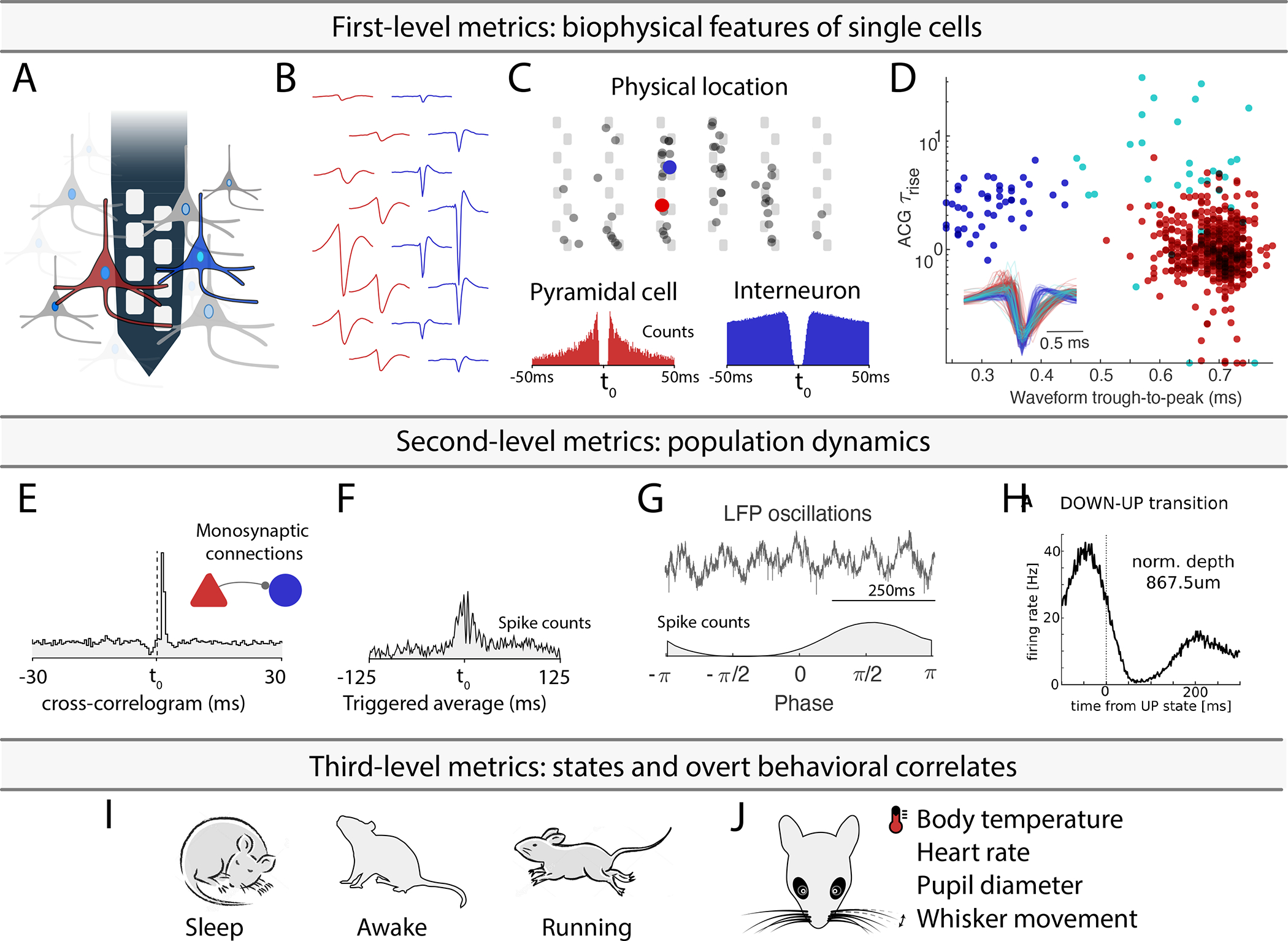
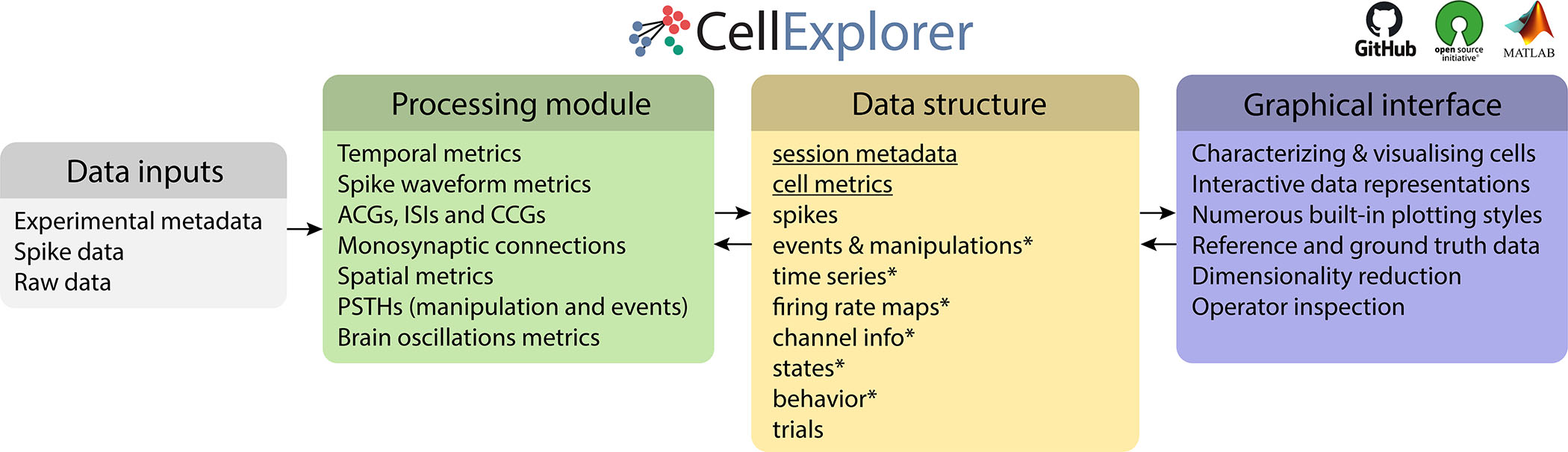
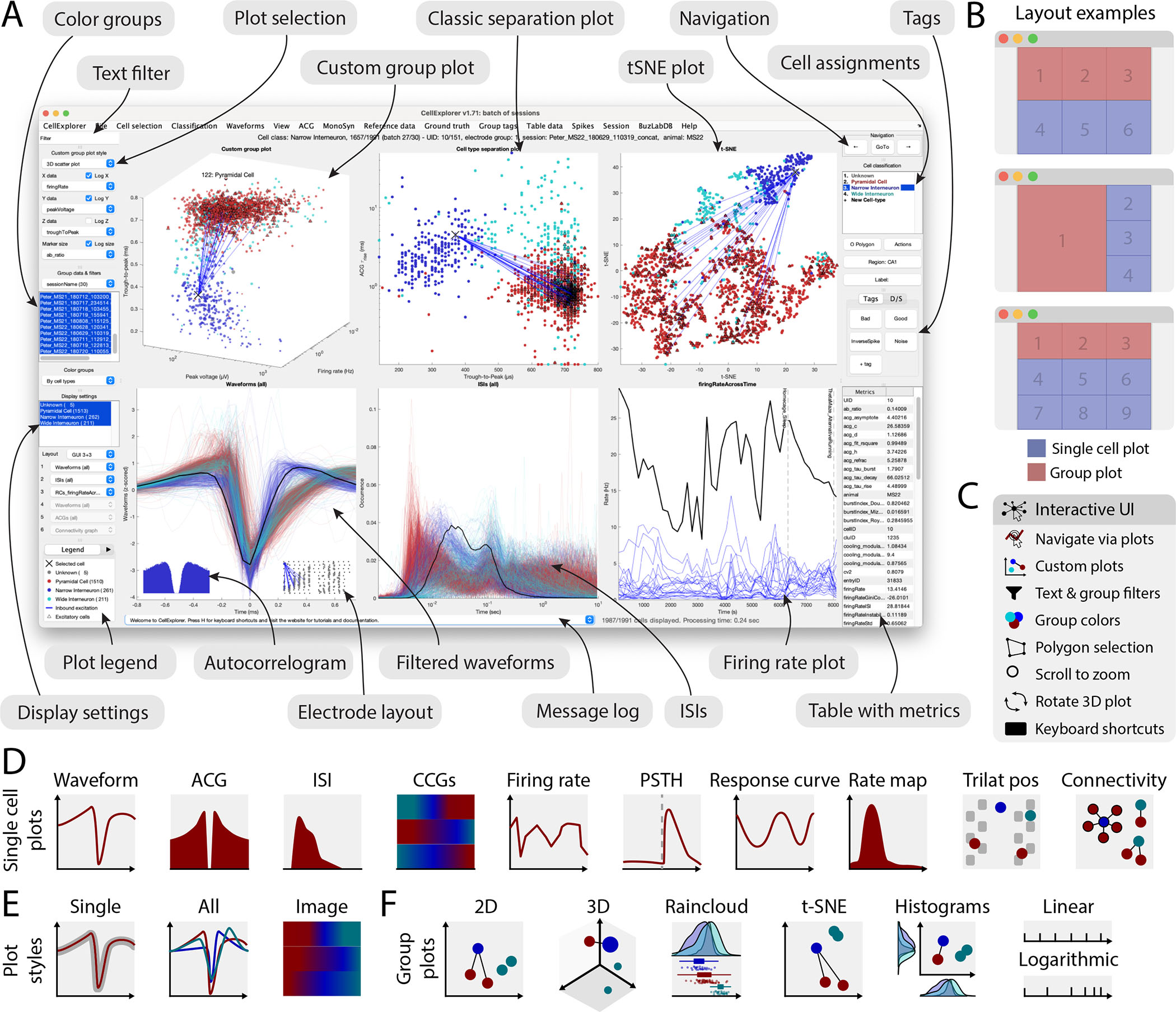
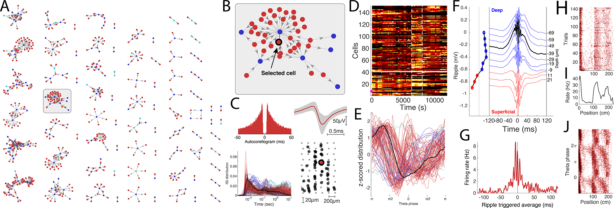
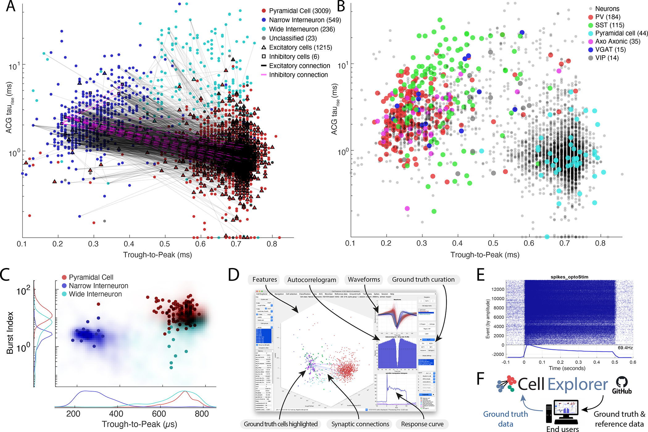
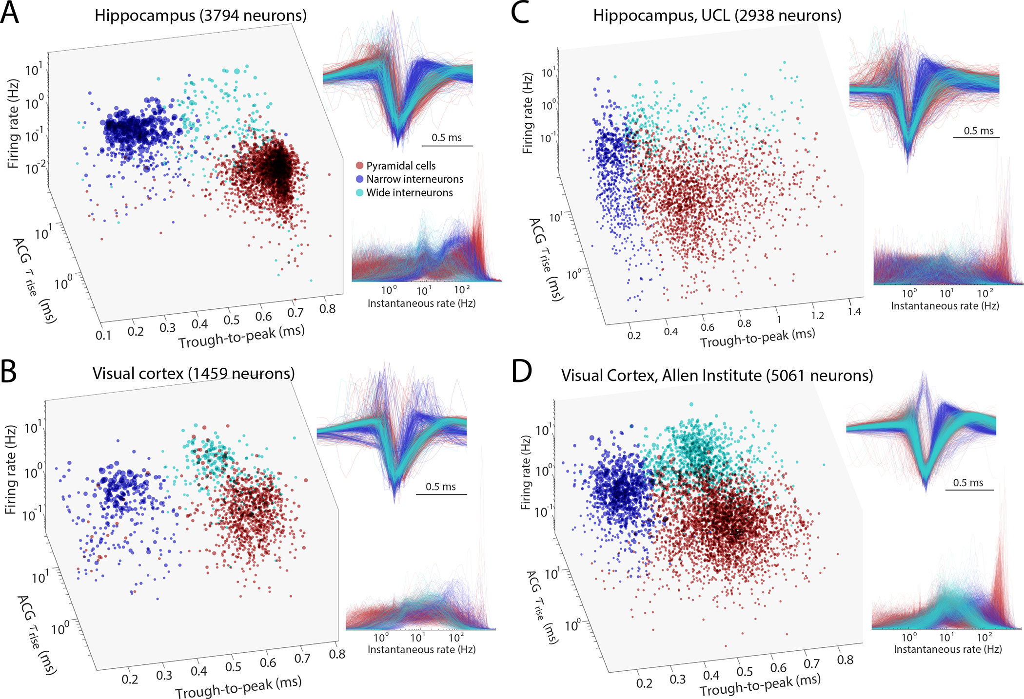
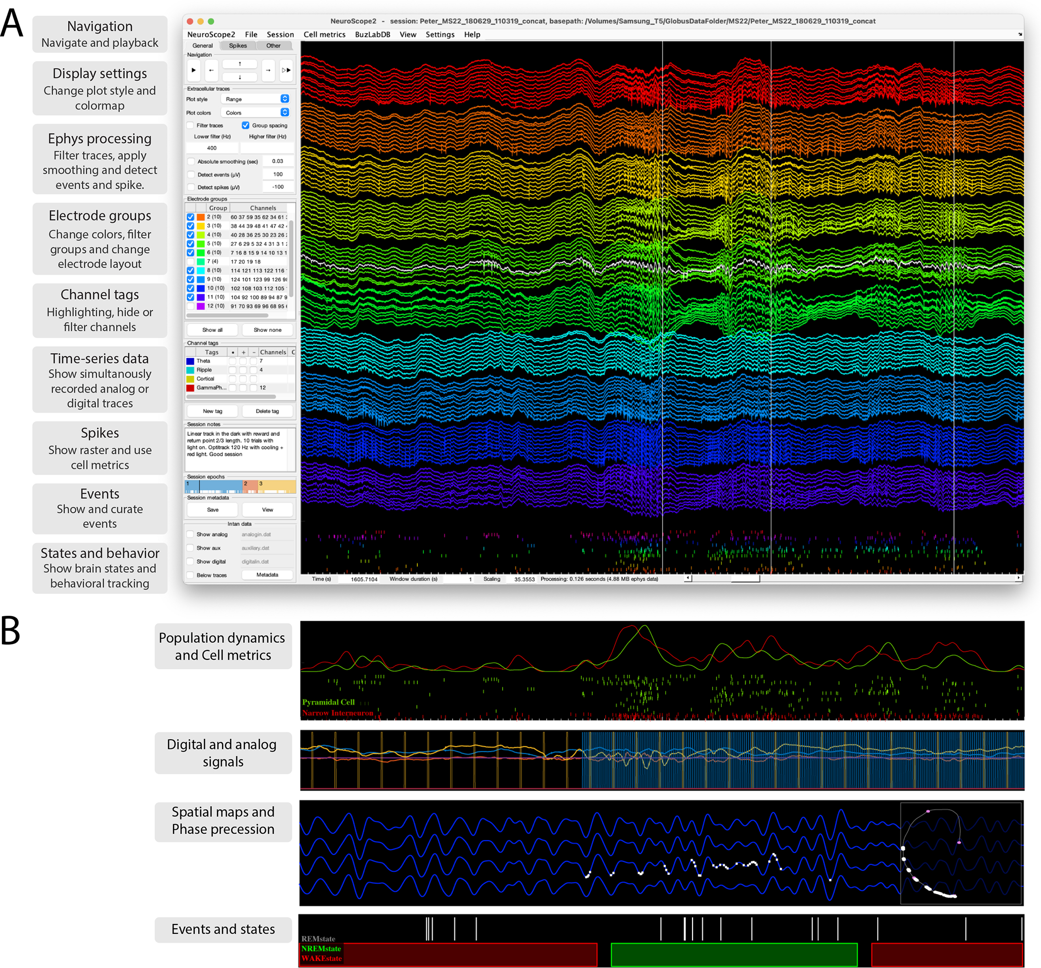
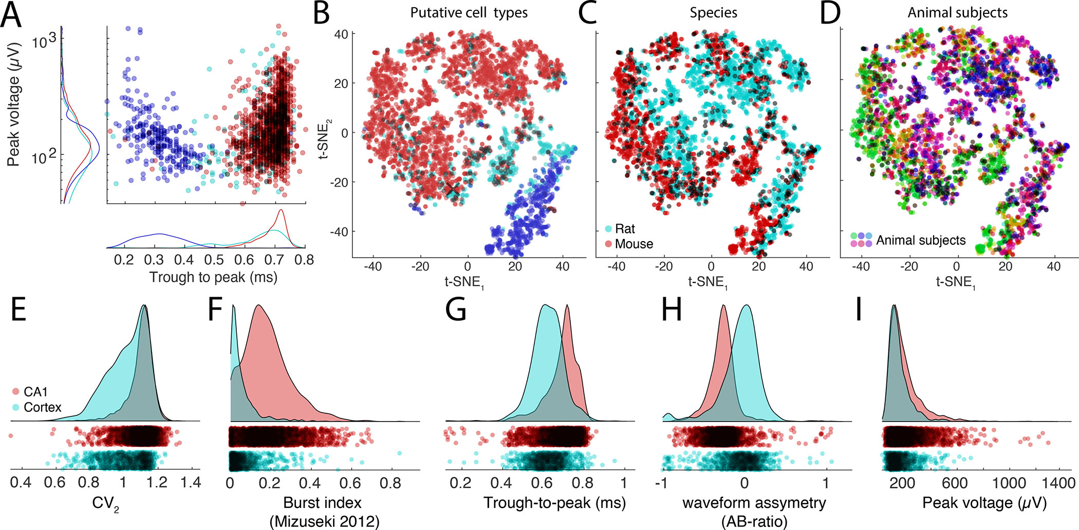
The large diversity of neuron types provides the means by which cortical circuits perform complex operations. Neuron can be described by biophysical and molecular characteristics, afferent inputs, and neuron targets. To quantify, visualize, and standardize those features, we developed the open-source, MATLAB-based framework CellExplorer. It consists of three components: a processing module, a flexible data structure, and a powerful graphical interface. The processing module calculates standardized physiological metrics, performs neuron-type classification, finds putative monosynaptic connections, and saves them to a standardized, yet flexible, machine-readable format. The graphical interface makes it possible to explore the computed features at the speed of a mouse click. The framework allows users to process, curate, and relate their data to a growing public collection of neurons. CellExplorer can link genetically identified cell types to physiological properties of neurons collected across laboratories and potentially lead to interlaboratory standards of single-cell metrics.

Keywords: electrophysiology; extracellular electrodes; framework; graphical interface; single cell analysis; standardized processing and data structure.

Figure 1:. Experimental paradigm-independent characterization of single neurons.

A. Using high-density silicon probes or multiple tetrodes (shown is a single shank with 8 recording sites), dozens to hundreds of neurons can be recorded simultaneously. B. Spikes of putative single neurons are extracted from the recorded traces and assigned to individual neurons through spike sorting algorithms. C. Their relative position determined through trilateration (the top panel shows neurons projected on a silicon probe with 6 shanks and a staggered electrode layout). Autocorrelograms (ACGs; lower two panels) are used to characterize the neurons (a bursting pyramidal cell with a wide waveform in red; a fast spiking interneuron with a narrow waveform in blue). D. Neuron-type classification based on first-order biophysical parameters, such as spike waveform width (trough-to-peak) and the temporal scale of the rising phase of the ACGs (τ_rise). Optogenetic and other direct identification methods can further ground units to neuron types. E. Interactions between neurons are characterized by their cross-correlograms and monosynaptic connections (determined via spike transmission probabilities). F. Event related histogram. G. Relating spikes to LFP patterns. H. Relating spikes to brain state changes. I-J. Spike pattern correlations with brain states and overt behaviors. Only a few possible examples are shown. See also Supplementary Table 1.

Figure 2.. Three-component framework.

A single extensive processing module (green); Standardized yet flexible data structure (yellow); and a graphical interface (purple). Data inputs are compatible with most existing spike sorting algorithms (grey). The data structure joins the Processing module with the Graphical interface (* signifies data containers). CellExplorer is open-source, built in MATLAB, and available on GitHub. See also Supplementary Figure 1, 2, 3 and Supplementary Table 2.

Figure 3:. Graphical interface.

A. The interface consists of 4 to 9 main plots, where the top row is dedicated to population-level representations of the neurons. Other plots are selectable and customizable for individual neuron (e.g., single waveforms, ACGs, ISIs, CCGs, PSTHs, response curves, and firing rate maps). The surrounding interface consists of panels placed on either side of the graphs. The left side displays settings and population settings, including a custom plot panel, color group panel, display settings panel, and legends. The right side-panel displays single-cell dimensions, including a navigation panel, neuron assignment panel, tags, and a table with metrics. In addition, there is a text filter and a message log. B. Layout examples highlighting three configurations with 1–3 group plots and 3–6 single neuron plots. C. The interface has many interactive elements, including navigation and selection from plots (left mouse click links to selected cell and right mouse click selects the neuron from all the plots), visualization of monosynaptic connections, various data plotting styles (more than 30+ unique plots built-in), supports custom plots; plotting filters can be applied by text or selection, keyboard shortcuts, zooming any plot by mouse-scrolling and polygon selection of neurons D. Single cell plot options: waveform, Autocorellogram (ACG), Inter-spike-interval (ISI), firing rate across time, Post-Stimulus Time Histogram (PSTH), response curve, spatial firing rate maps, trilaterated neuronal position relative to recording sites, and monosynaptic connectivity graph. E. Most single cell plots have three representations: individual single cell representation, single cell together with the entire population with absolute amplitude and a normalized image representation (colormap). F. Group plotting options: 2D, 3D, raincloud plot, t-SNE, and double histogram. Each dimension can be plotted on linear or logarithmic axes. See also Supplementary Figure 4, 5, 6 and Supplementary Video 1.

Figure 4.. Data exploration example.

A. Connectivity graph with monosynaptic modules found across multiple datasets. Neurons are color-coded by their putative cell types (pyramidal cells in red, narrow interneurons in blue and wide interneurons in cyan). B. Highlighted monosynaptic module with single pyramidal cell highlighted (arrow). C. First level metrics: Auto-correlogram, average waveform (top row; gray area signifies the noise level of the waveforms), ISI distributions, with the selected neuron in black, and the physical location of the neurons relative to the multi-shank silicon probe. D. Firing rate across time for the population, each neuron is normalized to its peak rate. The session consists of three behavioral epochs: pre-behavior sleep, behavior (track running), and post-behavior sleep (boundaries shown with dashed lines). E. Theta phase distribution for all neurons recorded in the same session (red, pyramidal cells; blue, interneurons) during locomotion with the selected neuron highlighted (black line). F. Average ripple waveform for the electrode sites on a single shank. The site of the selected neuron is highlighted (dashed black line). The polarity of the average sharp wave is used to determine the position of the neuron relative to the pyramidal layer in CA1. G. Ripple wave-triggered PSTH for the selected neuron aligned to the ripple peak. H. Trial-wise raster for the selected neuron in a maze. I. The average firing rate of the neuron across trials. J. Spike raster showing the theta phase relationship to the spatial location of the animal.

Figure 5.. Community-based collaborations allow for improved single neuron characterization.

A. Distribution of putative cell types (3657 cells), including their projections determined via spike-transmissions CCG curves (Petersen and Buzsáki, 2020; Petersen et al., 2020) Excitatory and inhibitory cells determined from monosynaptic connections are highlighted with black triangles and magenta squares respectively. The marginal distributions are shown both as counts and probability distributions. B. Example ACGs for the three cell types and the ACG fit (black line). C. Top row: Average peak-normalized ACGs of the three cell types. bottom row: Average waveform for the three cell types (z-scored). D. t-SNE representation of the same cell population. E. Lower two panels: agglomerative clusters of data with 2 (left panel) and 3 clusters (right panel). F. 407 optogenetically identified neurons, including PV (184), SST (115), pyramidal cells (44), axo-axonic (35), VGAT (15) and VIP cells (14) projected onto the same population of neurons as in A (Sources: Allen Institute and Buzsáki lab; English et al., 2017; Senzai et al., 2019; Siegle et al., 2021). G. Isolation distance in cluster space for the population shown in A and I. See also Supplementary Figure 7 and 8.

Figure 6.. Comparison of initial neuron classification by CellExplorer on large scale datasets from three different laboratories.

A. Data from hippocampus (Petersen and Buzsáki, 2020). B. Data from visual cortex (Senzai et al., 2019). C. Hippocampal and visual neurons selected from the UCL dataset (Steinmetz et al., 2019). D. Visual cortex cells from the Allen Institute (Siegle et al., 2021). Right panels across A-D: Z-scored waveforms across all neurons (top) and distribution of instantaneous rates (1/interspike intervals) across all neurons. A and B are based on long home cage (sleep) data (several hours), while C and D data are from short (~ 30 min) sessions in head-fixed, task-performing mice. See also Suppl. Fig. 8. Red, pyramidal cells; Blue, narrow waveform interneurons; Cyan, wide waveform interneurons.

Figure 7.. NeuroScope2 - A data viewer for raw and processed extracellular data acquired using multisite silicon probes, tetrodes or single wires.

NeuroScope2 is written in Matlab, maintaining many of the original features of NeuroScope (neurosuite.sourceforge.net), but with many enhancements, and it is faster. It is easy to hack or modify, and supports and relies on the data types of CellExplorer. A. Screenshot of the graphical interface, showing a 128-channel recording from the rat hippocampus (window duration = 1 sec). Each colored groups of traces are from the same shank. The three vertical lines are detected temporal events (sharp-wave ripples; detection-channel is highlighted in white). The rasters below the traces are the spikes from curated single units. The left side panel consists of three tabs: General (panels: navigation, ephys traces, electrode groups, channel tags, session notes and epochs, and intan time-series), Spikes (panels: spikes, cell metrics, population dynamics) and Other (panels: events, states, time-series, and behavioral data). B. Various visualizations with NeuroScope2. Top: Population average curves and spiking dynamics of the same population of cells as in A, but color coded and grouped using the putative cell type determined via CellExplorer (duration: 1 sec). Second panel: two digital TTL pulses and 3D accelerometer data (mounted on the animal’s head). Digital data captured using the Intan acquisition system (the TTLs pulses are emitted by a 10Hz camera and a 120Hz behavioral tracking systems; window duration: 3 sec). Third panel: Ephys traces filtered in the theta band, with spikes of a single place cell plotted on the same trace (white bars; window duration: 3 sec), the right square shows the animals spatial trajectory (grey line) and the white points indicate the spatial location of the place field. Lowest panel: Event rater and states data (window duration: 50 sec).

Figure 8.. Exploration and comparison of metrics and cells across, species, subjects and brain regions.

A. Distributions of spike amplitudes and waveform width (quantified by the trough to peak metrics) for the three groups from multiple CA1 datasets. Note inverse relationship between spike amplitude and waveform for putative interneurons. B-D. t-SNE representations of putative cell types (B), species (C, rat, and mouse in magenta and red, respectively) and subjects (D, colors scaled across subjects) for hippocampal neurons. E-I: Comparison of spike features of neurons recorded from CA1 pyramidal cells and visual cortex pyramidal cells. Significant differences are observed across several basic metrics, including CV₂ (E), burst index (F), trough-to-peak (G), waveform asymmetry (H), and waveform peak voltage (I).

References

1. Allen M, Poggiali D, Whitaker K, Marshall TR, van Langen J, and Kievit RA (2021). Raincloud plots: a multi-platform tool for robust data visualization. Wellcome Open Res 4, 63. - PMC - PubMed
1. Ascoli GA, Donohue DE, and Halavi M (2007). NeuroMorpho.Org: A Central Resource for Neuronal Morphologies. J Neurosci 27, 9247–9251. - PMC - PubMed
1. Barlow HB (1972). Single Units and Sensation: A Neuron Doctrine for Perceptual Psychology? Perception 1, 371–394. - PubMed
1. Barthó P, Hirase H, Monconduit L, Zugaro M, Harris KD, and Buzsáki G (2004). Characterization of neocortical principal cells and interneurons by network interactions and extracellular features. J. Neurophysiol. 92, 600–608. - PubMed
1. Bishop PO, Burke W, and Davis R (1962). Single-unit recording from antidromically activated optic radiation neurones. J Physiol 162, 432–450. - PMC - PubMed
Publication types
MeSH terms
LinkOut - more resources