A Hopf physical reservoir computer

Abstract

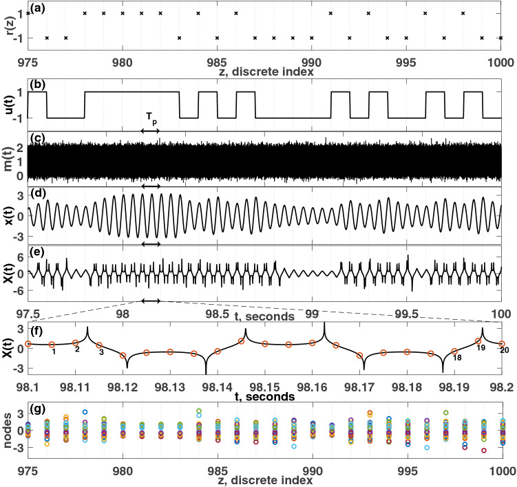
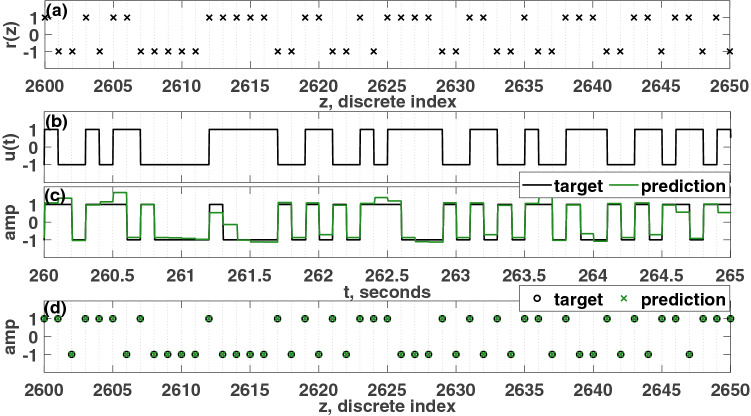
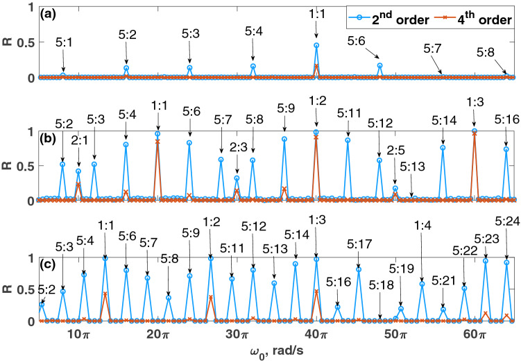
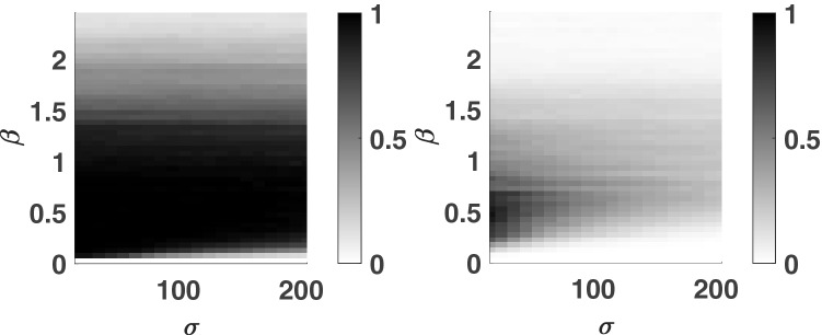
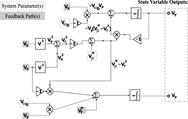
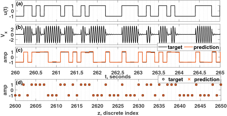
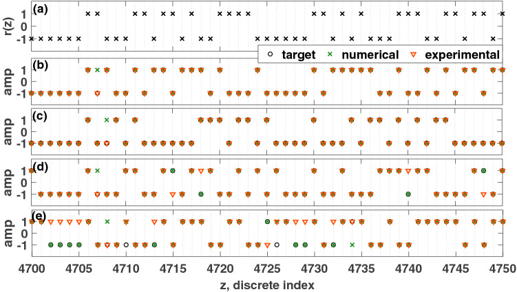
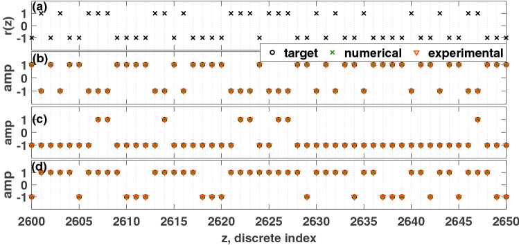
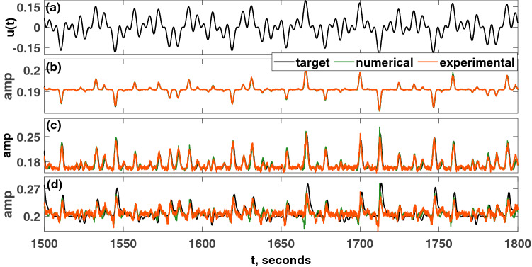
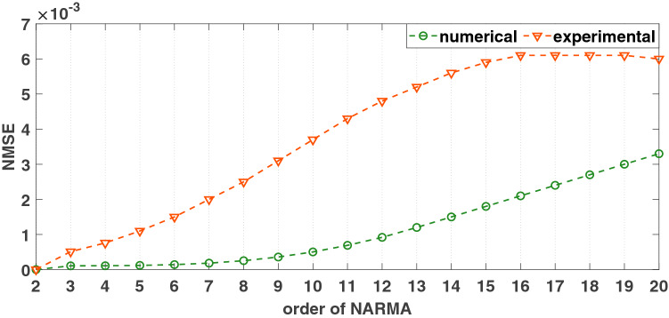
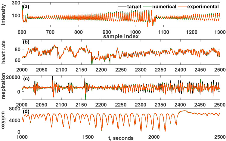
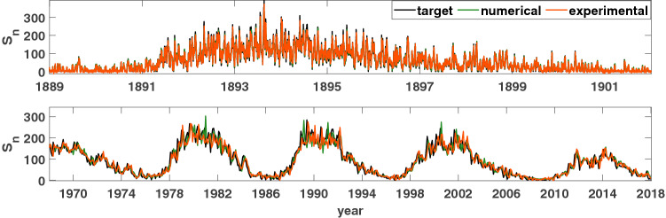
Physical reservoir computing utilizes a physical system as a computational resource. This nontraditional computing technique can be computationally powerful, without the need of costly training. Here, a Hopf oscillator is implemented as a reservoir computer by using a node-based architecture; however, this implementation does not use delayed feedback lines. This reservoir computer is still powerful, but it is considerably simpler and cheaper to implement as a physical Hopf oscillator. A non-periodic stochastic masking procedure is applied for this reservoir computer following the time multiplexing method. Due to the presence of noise, the Euler-Maruyama method is used to simulate the resulting stochastic differential equations that represent this reservoir computer. An analog electrical circuit is built to implement this Hopf oscillator reservoir computer experimentally. The information processing capability was tested numerically and experimentally by performing logical tasks, emulation tasks, and time series prediction tasks. This reservoir computer has several attractive features, including a simple design that is easy to implement, noise robustness, and a high computational ability for many different benchmark tasks. Since limit cycle oscillators model many physical systems, this architecture could be relatively easily applied in many contexts.

Figure 1

(a) Discrete random binary signal, r(z). (b) Continuous input signal, u(t). (c) Stochastic masking function, m(t). (d) Time history of x(t). (e) Rescaled time history, X(t). (f) 20 equidistant nodes for a single pseudo-period, $T_p$, are denoted with circles. (g) Collected nodal states from the nodes for machine learning input data set. Different colors in (g) denote different nodes. For the simulation depicted here, the parameters were set such that: $\mu =5$, $A=0.5$, $\mathrm{\Omega }=40\pi$ rad/s, ${\omega }_0=40\pi$ rad/s, $T_p=0.1$ seconds, $N=20$ nodes, $\varphi =\pi /3$ rad, $\sigma =100$, $\beta =1.0$.

Figure 2

(a) Discrete random binary signal, r(z). (b) Continuous input signal, u(t). (c) target signal and continuous prediction. d) Discretized target and prediction. The calculated information metric is $R=0.98$. For the simulation depicted here, the parameters were set such that: $\mu =5$, $A=0.5$, $\mathrm{\Omega }=40\pi$ rad/s, ${\omega }_0=40\pi$ rad/s, $T_p=0.1$ s, $N=20$, $\varphi =\pi /3$ rad, $\sigma =100$, $\beta =1.0$.

Figure 3

Comparison of the reservoir’s computing performance, R, on the choice of the pseudo-period, $T_p$, and the natural frequency, ${\omega }_0$ using 2nd and 4th order parity tasks. (a) $T_p=0.05$ seconds, (b) $T_p=0.1$ seconds, and (c) $T_p=0.15$ seconds. Different ratios of the natural period and pseudo-period (e.g., $\frac{2\pi }{{\omega }_0}:T_p$) are simulated, and the ratios are depicted for peaks in the information metric. ${\omega }_0=\mathrm{\Omega }=50\pi$ rad/s is the resonance case. Parameters were set such that: $\mu =5$, $A=0.5$, $\mathrm{\Omega }=50\pi$ rad/s, $N=1000$ nodes, $\varphi =\pi /3$ rad, $\sigma =15$, $\beta =1.0$.

Figure 4

The reservoir computer is somewhat robust to noise. The effects of $\sigma$ and $\beta$ are shown. Left: 4th order parity task. Right: 6th order parity task. Parameters were set such that: $\mu =5$, $A=0.5$, $\mathrm{\Omega }=40\pi$ rad/s, ${\omega }_0=40\pi$ rad/s, $T_p=0.1$ seconds, $N=1000$ nodes, and $\varphi =\pi /3$ rad.

Figure 5

A simplified schematic for the Hopf PRC, with states $V_x$ and $V_y$. $V_{\mu }^e=V_{\mu }(1+V_u{V}_m)$ and $V_f^e=A(1+V_u{V}_m)sin(\mathrm{\Omega }t+\varphi )$.

Figure 6

(a) Input voltage signal, $V_u$. (b) Time history of $V_x$. (c) XOR target signal, M, and the prediction. (d) Discretized prediction. The calculated information metric is $R=1.0$. For the experimental results depicted here, the parameters were set such that: $V_{\mu }=5$ volts, $A=0.5$ volts, $\mathrm{\Omega }=40\pi$ rad/s, $V_{{\omega }_0}=40\pi$ volts, $T_p=0.1$ seconds, $N=20$ nodes, $\varphi =\pi /3$ rad, $\sigma =10$ volts, $\beta =1.0$ volts.

Figure 7

Comparison of the performance of the PRC for parity tasks. (a) Discrete input function, r(z). (b) 2nd order parity task. Information metric: $R_{\mathit{exp}}=1.00$, $R_{\mathit{sim}}=0.98$. (c) 3rd order parity task. Information metric: $R_{\mathit{exp}}=1.00$, $R_{\mathit{sim}}=0.98$. (d) 4th order parity task. Information metric: $R_{\mathit{exp}}=0.68$, $R_{\mathit{sim}}=0.93$. (e) 5th order parity task. Information metric: $R_{\mathit{exp}}=0.31$, $R_{\mathit{sim}}=0.74$. Parameters were set such that: $V_{\mu }=\mu =5$, $A=0.5$, $\mathrm{\Omega }=40\pi$ rad/s, $V_{{\omega }_0}={\omega }_0=40\pi$, $T_p=0.1$ seconds, $N=1000$ nodes, $\varphi =\pi /3$ rad, $\sigma =15$, $\beta =1.0$, and a total time of $5000T_p=500$ seconds (only a portion of the discrete prediction is shown).

Figure 8

Comparison of the performance of the PRC for parity tasks. (a) Input function, u(t). (b) NOT ($\neg$) gate. (c) AND ($\wedge$) gate, (d) OR ($\vee$) gate. For all numerical and experimental results, the information rate was at the theoretical maximum; the Hopf PRC can act as any of the fundamental logic gates. Parameters were set such that: $V_{\mu }=\mu =5$, $A=0.5$, $\mathrm{\Omega }=40\pi$ rad/s, $V_{{\omega }_0}={\omega }_0=40\pi$ rad/s, $T_p=0.1$ seconds, $N=1000$ nodes, $\varphi =\pi /3$ rad, $\sigma =15$, $\beta =1.0$, and a total time of $3000T_p=300$ seconds. Only a portion of the response is shown here.

Figure 9

Comparison of the performance of the PRC for NARMA tasks. (a) Input function, u(t). (b) 2nd order NARMA task. Performance metric: $NMS{E}_{\mathit{exp}}=2.8181\times {10}^{-6}$, $NMS{E}_{\mathit{sim}}=7.8199\times {10}^{-7}$. (c) 10th order NARMA task. $NMS{E}_{\mathit{exp}}=0.0037$, $NMS{E}_{\mathit{sim}}=5.0362\times {10}^{-4}$. (d) 20th order NARMA task. $NMS{E}_{\mathit{exp}}=0.0060$, $NMS{E}_{\mathit{sim}}=0.0033$. Only a portion of the result is shown in each figure. Parameters were set such that: $V_{\mu }=\mu =5$, $A=0.5$, $\mathrm{\Omega }=40\pi$ rad/s, $V_{{\omega }_0}={\omega }_0=40\pi$, $T_p=0.1$ seconds, $N=1000$ nodes, $\varphi =\pi /3$ rad, $\sigma =15$, $\beta =1.0$.

Figure 10

Plot of the NMSE of the 2nd to 20th order NARMA tasks for the simulation and experiment. Parameters were set such that: $V_{\mu }=\mu =5$, $A=0.5$, $\mathrm{\Omega }=40\pi$ rad/s, $V_{{\omega }_0}={\omega }_0=40\pi$, $T_p=0.1$ seconds, $N=1000$, $\varphi =\pi /3$ rad, $\sigma =15$, $\beta =1.0$.

Figure 11

Comparison of the performance of the PRC for Santa Fe prediction tasks. (a) The Santa Fe chaotic time series of a laser intensity prediction task. Performance metric: $NMS{E}_{\mathit{exp}}=0.0615$, $NMS{E}_{\mathit{sim}}=0.02$. (b) The Santa Fe heart rate prediction task. $NMS{E}_{\mathit{exp}}=6.0258\times {10}^{-4}$, $NMS{E}_{\mathit{sim}}=6.5060\times {10}^{-4}$. (c) Santa Fe respiration force prediction task. $NMS{E}_{\mathit{exp}}=0.1826$, $NMS{E}_{\mathit{sim}}=0.1753$. (d) Santa Fe blood oxygen concentration prediction task. $NMS{E}_{\mathit{exp}}=3.3287\times {10}^{-4}$, $NMS{E}_{\mathit{sim}}=1.7\times {10}^{-4}$. Parameters were set such that: $V_{\mu }=\mu =5$ volts, $A=0.5$ volts, $\mathrm{\Omega }=40\pi$ rad/s, $V_{{\omega }_0}={\omega }_0=40\pi$ volts, $T_p=0.1$ seconds, $N=1000$ nodes, $\varphi =\pi /3$ rad, $\sigma =15$ volts, $\beta =1.0$ volts. Only a portion of the result is shown in each figure.

Figure 12

Comparison of the performance the sunspot prediction ($S_n$) task. Top: Daily total number of sunspot prediction task, for both the experiment and the numerical simulations. Performance metric: $NMS{E}_{\mathit{exp}}=0.0548$, $NMS{E}_{\mathit{sim}}=0.0534$. Bottom: Monthly mean total number of sunspot prediction task. Performance metric: $NMS{E}_{\mathit{exp}}=0.0595$, $NMS{E}_{\mathit{sim}}=0.0455$. Parameters were set such that: $V_{\mu }=\mu =5$ volts, $A=0.5$ volts, $\mathrm{\Omega }=40\pi$ rad/s, $V_{{\omega }_0}={\omega }_0=40\pi$ rad/s, $N=1000$ nodes, $\varphi =\pi /3$ rad, $\sigma =15$ volts, $\beta =1.0$ volts. Only a portion of the result is shown in each figure.

References

1. Jaeger H, Haas H. Harnessing nonlinearity: Predicting chaotic systems and saving energy in wireless communication. Science. 2004;304:78–80. doi: 10.1126/science.1091277. - DOI - PubMed
1. Lukoševičius M, Jaeger H. Reservoir computing approaches to recurrent neural network training. Comput. Sci. Rev. 2009;3:127–149. doi: 10.1016/j.cosrev.2009.03.005. - DOI
1. Nakajima K. Physical reservoir computing-an introductory perspective. Jpn. J. Appl. Phys. 2020;59:060501. doi: 10.35848/1347-4065/ab8d4f. - DOI
1. Nakajima K, Hauser H, Li T, Pfeifer R. Information processing via physical soft body. Sci. Rep. 2015;5:10487. doi: 10.1038/srep10487. - DOI - PMC - PubMed
1. Haynes ND, Soriano MC, Rosin DP, Fischer I, Gauthier DJ. Reservoir computing with a single time-delay autonomous boolean node. Phys. Rev. E. 2015;91:020801. doi: 10.1103/PhysRevE.91.020801. - DOI - PubMed