A cross-population atlas of genetic associations for 220 human phenotypes

Abstract

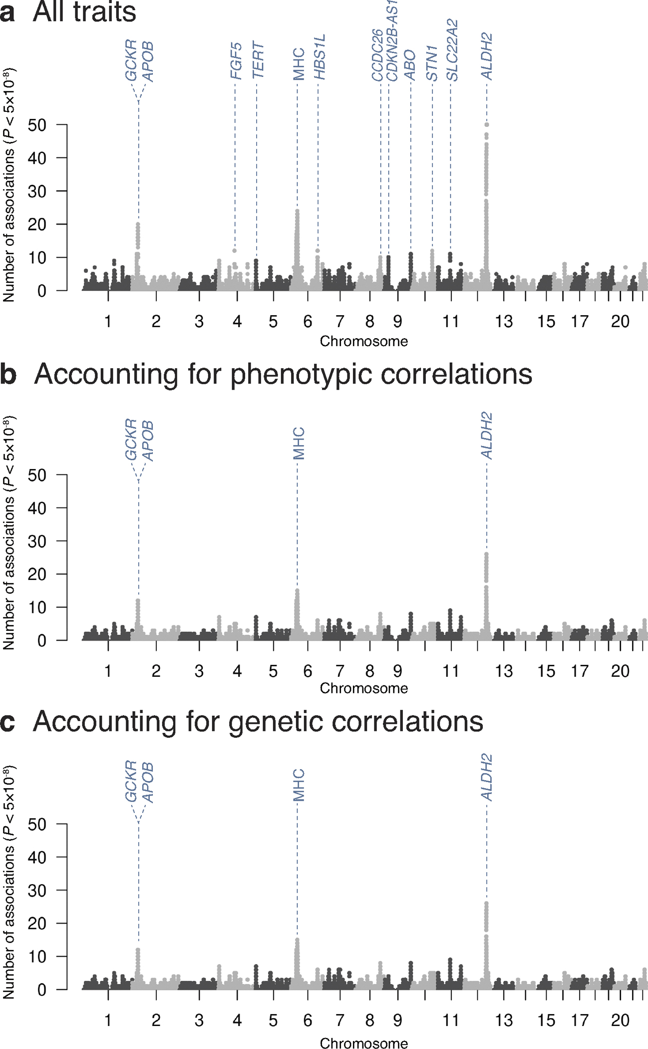
Current genome-wide association studies do not yet capture sufficient diversity in populations and scope of phenotypes. To expand an atlas of genetic associations in non-European populations, we conducted 220 deep-phenotype genome-wide association studies (diseases, biomarkers and medication usage) in BioBank Japan (n = 179,000), by incorporating past medical history and text-mining of electronic medical records. Meta-analyses with the UK Biobank and FinnGen (n_total = 628,000) identified ~5,000 new loci, which improved the resolution of the genomic map of human traits. This atlas elucidated the landscape of pleiotropy as represented by the major histocompatibility complex locus, where we conducted HLA fine-mapping. Finally, we performed statistical decomposition of matrices of phenome-wide summary statistics, and identified latent genetic components, which pinpointed responsible variants and biological mechanisms underlying current disease classifications across populations. The decomposed components enabled genetically informed subtyping of similar diseases (for example, allergic diseases). Our study suggests a potential avenue for hypothesis-free re-investigation of human diseases through genetics.

Extended Data Fig. 1. Overview of this study.

We performed 220 deep-phenotype GWASs in BioBank Japan, including 108 novel GWASs ever conducted in East Asian population. We performed trans-biobank meta-analyses with UK Biobank and FinnGen (n_total = 628,000), resulting in discovery of 5,343 novel loci. All summary statistics are openly shared through pheweb.jp web portal. As downstream analyses, we performed (i) cross-population comparison of pleiotropy and genetic correlation, (ii) comprehensive HLA fine-mapping, and (iii) statistical decomposition of a matrix of summary statistics to gain insights into biology underlying current disease classifications, by incorporating functional genomics, metabolomics, and biomarker data.

Extended Data Fig. 2. Locus plots for representative loci.

(a) Regional association plots for Pulmonary Tuberculosis (PTB) in BBJ are shown. The lead variant (rs140780894) is colored in pink, and colors of other dots indicate linkage disequilibrium measure r² with the lead variant. (b) Regional association plots for cholelithiasis in BBJ are shown. The lead variant (rs715) is colored in pink, and colors of other dots indicate linkage disequilibrium measure r² with the lead variant. (c) Regional association plots for gastric diseases in BBJ at the PSCA locus in gastric ulcer, gastric cancer, and gastric polyp are shown. Rs2976397, which was a lead variant in gastric ulcer, is colored in pink, and colors of other dots indicate linkage disequilibrium measure r² with the lead variant. (d) Regional association plots at the FUT3 locus in gall bladder polyp and cholelithiasis in BBJ are shown. Rs28362459, which was a lead variant in gall bladder polyp, is colored in pink, and colors of other dots indicate linkage disequilibrium measure r² with the lead variant. (e) Regional association plots for urticaria in BBJ are shown. The lead variant (rs56043070) is colored in pink, and colors of other dots indicate linkage disequilibrium measure r² with the lead variant. (f) Regional association plots for salicylic acids prescription in BBJ are shown. The lead variant (rs151193009) is colored in pink, and colors of other dots indicate linkage disequilibrium measure r² with the lead variant.

Extended Data Fig. 3. The effect size correlation between BBJ GWAS and European GWAS.

The marginal effect sizes of genome-wide significant variants across traits in BBJ are compared with those in European GWAS. Each plot represents a variant, and is colored based on the significance in European GWAS as shown in the left top legend. Pearson’s correlation r and P value (two-sided) between BBJ GWAS and European GWAS are also shown in the legend.

Extended Data Fig. 4. Phenotypic correlation across 220 phenotypes in BBJ.

a. Heatmap of pair-wise phenotypic correlation matrix. The color of the cells indicates the value of correlation r as shown in a color scale at the bottom. The traits (rows and columns) were hierarchically clustered by hclust library in R. b. Silhouette score for clustering of closely related phenotypes with different number of clusters (Supplementary Notes).

Extended Data Fig. 5. The degree of pleiotropy in BBJ after accounting for phenotypic or genetic correlations.

The Manhattan-like plots show the number of significant associations (P < 5.0×10⁻⁸) at each tested genetic variant in Japanese. a. For all traits (n_trait = 220; as shown in Fig. 2a). b. After accounting for phenotypic correlations. c. After accounting for genetic correlations.

Extended Data Fig. 6. Genetic correlation matrices across populations.

The matrices describe pairwise genetic correlation r_g in Japanese GWAS (a; n = 5,565) and in European GWAS (b; n = 10,878), which was estimated by bivariate LD score regression. A color of the cells indicates the value of r_g as shown in a color scale at the bottom. The traits (rows and columns) were hierarchically clustered by hclust library in R, and trait domains are displayed as colored boxes (see Methods).

Extended Data Fig. 7. Network representation of the TSVD analysis.

Two-dimensional illustration of interconnection among 159 diseases and 40 latent components. Plots in blue indicate each trait’s statistics, and plots in pink indicate the latent components derived by TSVD. White lines represent the contribution of each phenotype in each component. The width of the lines indicates the strength of the contribution based on the squared cosine score.

Extended Data Fig. 8. Heatmap representation of squared cosine scores of diseases to components.

The components (rows) are shown from 1 (top) to 40 (bottom), and the diseases (columns) are sorted based on the contribution of each component to the disease based on the squared cosine score (from component 1 to 40). Each cell is colored based on the squared cosine score of a given trait to a given component, as shown in a color scale at the bottom right.

Extended Data Fig. 9. Enrichment analyses of genes explaining each component with tissue specificity.

A heatmap representation of the enrichment analyses of genes explaining each component with tissue-specific genes defined by GTEx expression profile (a) and regulatory vocabulary from ENCODE3 data (b). Each cell is colored based on P_enrichment from Fisher’s exact tests to assess the enrichment of the genes comprising each component within each tissue-specific gene set as shown in a color scale at the bottom right.

Extended Data Fig. 10. Genetic variants analyzed in the three cohorts.

The Venn diagram showing the number of genetic variants analyzed in this study in each of the three cohorts (BBJ, UKB, and FinnGen) and overlapping variants across the cohorts.

Figure 1.. Overview of the identified loci in the cross-population meta-analyses of 220 deep phenotype GWASs.

(a-c) The pie charts describe the phenotypes analyzed in this study. The disease endpoints (a; n_trait=159) were categorized based on the International Classification of Diseases (ICD)10 classifications (A to Z; Supplementary Table 1a), the biomarkers (b; n_trait=38; Supplementary Table 1b) were classified into nine categories, and medication usage was categorized based on the Anatomical Therapeutic Chemical Classification (ATC) system (A to S; Supplementary Table 1c). (d) The genome-wide significant loci identified in the cross-population meta-analyses and pleiotropic loci (P<5.0×10⁻⁸). The traits (rows) are sorted as shown in the pie chart, and each dot represents significant loci in each trait. Pleiotropic loci are annotated by lines with a locus symbol.

Figure 2.. Number of significant associations per variant.

(a, b) The Manhattan-like plots show the number of significant associations (P<5.0×10⁻⁸) at each tested genetic variant for all traits (n_trait=220) in Japanese (a) and in European GWASs (b). Loci with a large number of associations were annotated based on the closest genes of each variant. (c, d) The plots indicate the fold change of the sum of singleton density score (SDS) χ² within variants with a larger number of significant associations than a given number on the x-axis compared with those under the null hypothesis in Japanese (c) and in Europeans (d). We also illustrated a regression line based on local polynomial regression fitting.

Figure 3.. HLA and ABO association PheWAS.

(a,b) Significantly associated HLA genes identified by HLA PheWAS in BioBank Japan (BBJ; a) or in UK Biobank (UKB; b) are plotted (P<5.0×10⁻⁸). In addition to primary association signals of the phenotypes, independent associations identified by conditional analyses are also plotted, and the primary association is indicated by the plots with a gray border. The color of each plot indicates two-tailed P values calculated with logistic regression (for binary traits) or linear regression (for quantitative traits) as designated in the color bar at the bottom. The bars in green at the top indicate the number of significant associations per gene in each of the populations. The detailed allelic or amino acid position as well as statistics in the association are provided in Supplementary Table 8. (c,d) Significant associations identified by ABO blood-type PheWAS in BBJ (c) or in UKB (d) are shown as boxes and colored based on the odds ratio. The size of each box indicates two-tailed P values calculated with logistic regression (for binary traits) or linear regression (for quantitative traits).

Figure 4.. The deconvolution analysis of a matrix of summary statistics of 159 diseases across populations.

(a) An illustrative overview of deconvolution-projection analysis. Using DeGAs framework, a matrix of summary statistics from two populations (EUR: European and BBJ: Biobank Japan) was decomposed into latent components, which were interpreted by annotation of a set of genetic variants driving each component and in the context of other GWASs through projection. (b) A schematic representation of truncated singular-value decomposition (TSVD) applied to decompose a summary statistic matrix $\mathbf{W}$ to derive latent components. $\mathbf{U}$, $\mathbf{S}$, and $\mathbf{V}$ represent resulting matrices of singular values ($\mathbf{S}$) and singular vectors ($\mathbf{U}$ and $\mathbf{V}$). (c) A heatmap representation of DeGAs squared cosine scores of diseases (columns) to components (rows). The components are shown from 1 (top) to 40 (bottom), and diseases are sorted based on the contribution of each component to the disease measured by the squared cosine score (from component 1 to 40). Full results with disease and component labels are in Extended Data Figure 8. (d) Results of TSVD of disease genetics matrix and the projection of biomarker genetics. Diseases (left) and biomarkers (right) are colored based on the ICD10 classification and functional categorization, respectively. The derived components (middle; from 1 to 40) are colored alternately in blue or red. The squared cosine score of each disease to each component and each biomarker to each component is shown as red and blue lines. The width of the lines indicates the degree of contribution. The diseases with squared cosine score>0.3 in at least one component are displayed. Anth; anthropometry, BP; blood pressure, Metab; metabolic, Prot; protein, Kidn; kidney-related, Ele; Electrolytes, Liver; liver-related, Infl; Inflammatory, BC; blood cell.

Figure 5.. Examples of disease-component correspondence and biological interpretation of the components by projection and enrichment analysis using GREAT.

Shown is a representative component explaining a group of diseases based on the contribution score, along with responsible genes, functional enrichment results by GREAT, relevant tissues, and relevant biobarkers/metabolites. (a) The functional annotation of gall bladder related diseases and the component 10. GB; gallbladder. (b) The functional annotation of varicose vein and the component 11. (c) The functional annotation of autoimmune diseases and the component 27. RA; rheumatoid arthritis. SLE; systemic lupus erythematosus. (d) The characterization of allergic diseases based on the components 3, 16, 26, and 34. The red bars indicate the sum of squared cosine scores of components 3 and 16 (axis-1), whereas the blue bars indicate the sum of squared cosine scores of components 26 and 34 (axis-2). We also performed functional characterization of those components by projection analysis and GREAT enrichment analysis.

References

1. Berger D A brief history of medical diagnosis and the birth of the clinical laboratory. Part 1--Ancient times through the 19th century. MLO. Med. Lab. Obs. 31, (1999). - PubMed
1. Organización Mundial de la Salud. International statistical classification of diseases and related health problems, 10th revision (ICD-10). World Heal. Organ. (2016).
1. Denny JC et al. Systematic comparison of phenome-wide association study of electronic medical record data and genome-wide association study data. Nat. Biotechnol. 31, 1102–1110 (2013). - PMC - PubMed
1. Welter D et al. The NHGRI GWAS Catalog, a curated resource of SNP-trait associations. Nucleic Acids Res. 42, D1001–6 (2014). - PMC - PubMed
1. Denny JC et al. PheWAS: Demonstrating the feasibility of a phenome-wide scan to discover gene-disease associations. Bioinformatics 26, 1205–1210 (2010). - PMC - PubMed
Method Only References
1. Sakaue S et al. Trans-biobank analysis with 676,000 individuals elucidates the association of polygenic risk scores of complex traits with human lifespan. Nat. Med. 26, 542–548 (2020). - PubMed
1. McLaren W et al. The Ensembl Variant Effect Predictor. Genome Biol. 17, 122 (2016). - PMC - PubMed
1. Willer CJ, Li Y & Abecasis GR METAL: Fast and efficient meta-analysis of genomewide association scans. Bioinformatics 26, 2190–2191 (2010). - PMC - PubMed
1. Brown BC, Ye CJ, Price AL & Zaitlen N Transethnic Genetic-Correlation Estimates from Summary Statistics. Am. J. Hum. Genet. 99, 76–88 (2016). - PMC - PubMed
1. Raychaudhuri S et al. Five amino acids in three HLA proteins explain most of the association between MHC and seropositive rheumatoid arthritis. Nat. Genet. 44, 291–296 (2012). - PMC - PubMed
Publication types