Identification, visualization, statistical analysis and mathematical modeling of high-feedback loops in gene regulatory networks

Abstract

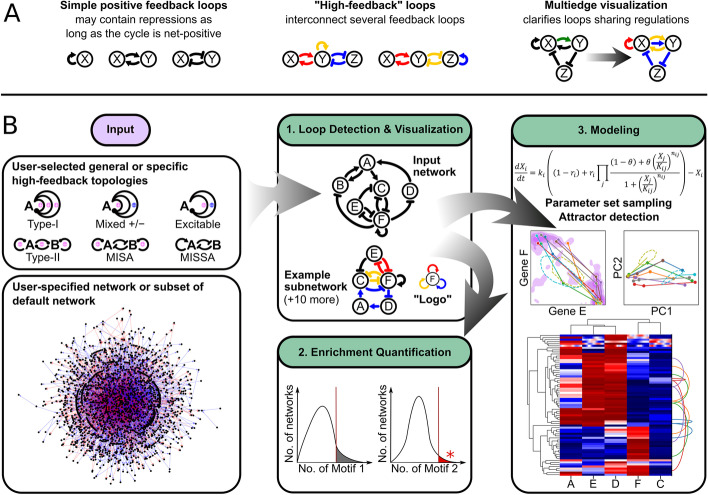
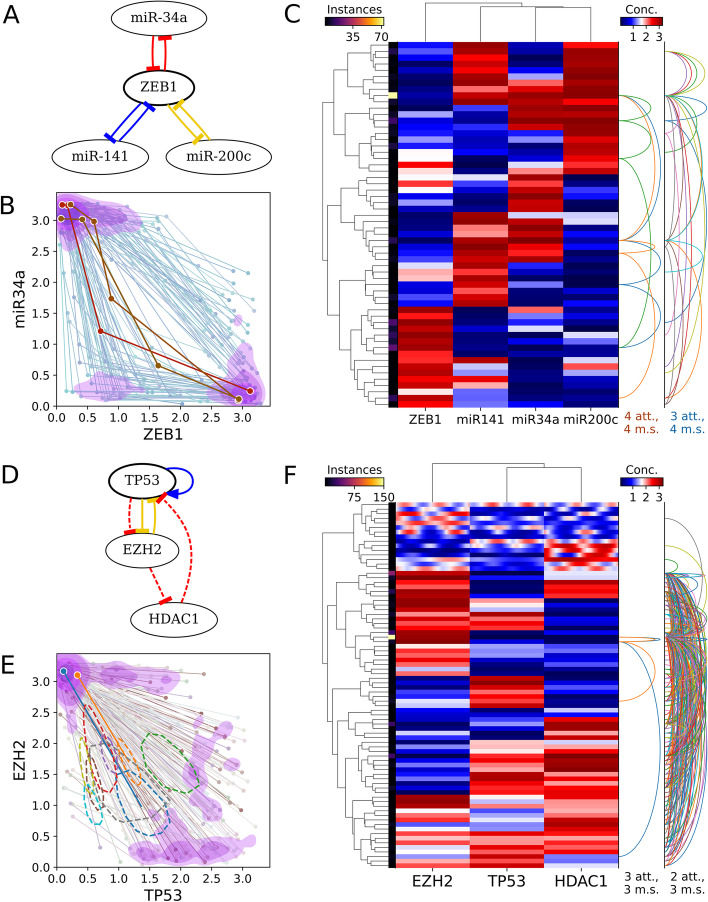
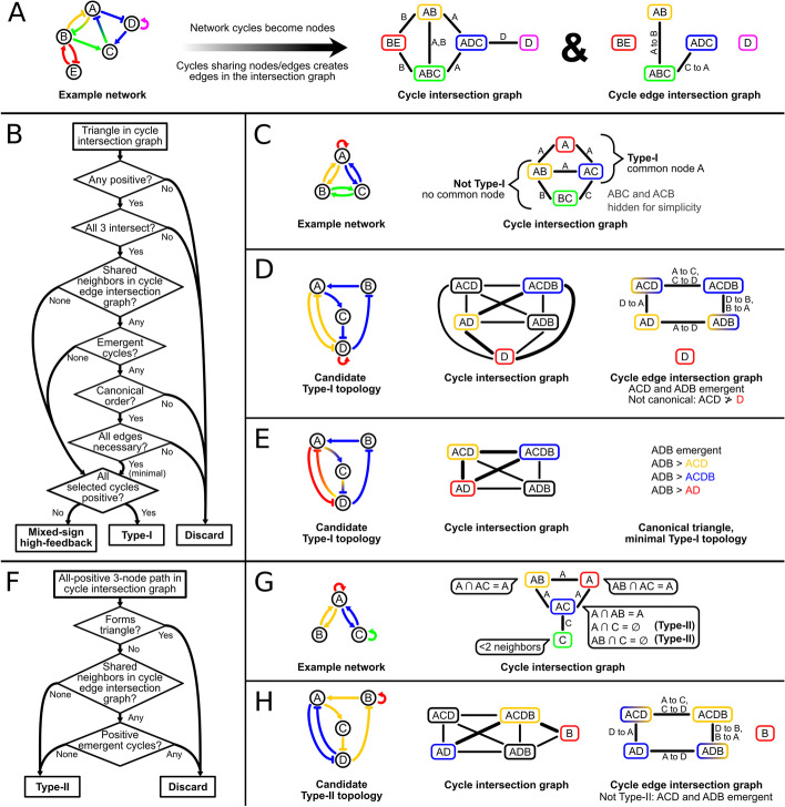
Background: Feedback loops in gene regulatory networks play pivotal roles in governing functional dynamics of cells. Systems approaches demonstrated characteristic dynamical features, including multistability and oscillation, of positive and negative feedback loops. Recent experiments and theories have implicated highly interconnected feedback loops (high-feedback loops) in additional nonintuitive functions, such as controlling cell differentiation rate and multistep cell lineage progression. However, it remains challenging to identify and visualize high-feedback loops in complex gene regulatory networks due to the myriad of ways in which the loops can be combined. Furthermore, it is unclear whether the high-feedback loop structures with these potential functions are widespread in biological systems. Finally, it remains challenging to understand diverse dynamical features, such as high-order multistability and oscillation, generated by individual networks containing high-feedback loops. To address these problems, we developed HiLoop, a toolkit that enables discovery, visualization, and analysis of several types of high-feedback loops in large biological networks.

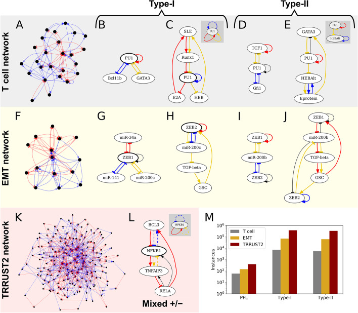
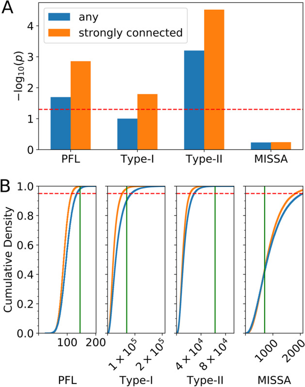
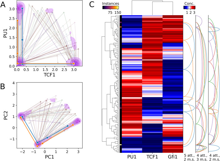
Results: HiLoop not only extracts high-feedback structures and visualize them in intuitive ways, but also quantifies the enrichment of overrepresented structures. Through random parameterization of mathematical models derived from target networks, HiLoop presents characteristic features of the underlying systems, including complex multistability and oscillations, in a unifying framework. Using HiLoop, we were able to analyze realistic gene regulatory networks containing dozens to hundreds of genes, and to identify many small high-feedback systems. We found more than a 100 human transcription factors involved in high-feedback loops that were not studied previously. In addition, HiLoop enabled the discovery of an enrichment of high feedback in pathways related to epithelial-mesenchymal transition.

Conclusions: HiLoop makes the study of complex networks accessible without significant computational demands. It can serve as a hypothesis generator through identification and modeling of high-feedback subnetworks, or as a quantification method for motif enrichment analysis. As an example of discovery, we found that multistep cell lineage progression may be driven by either specific instances of high-feedback loops with sparse appearances, or generally enriched topologies in gene regulatory networks. We expect HiLoop's usefulness to increase as experimental data of regulatory networks accumulate. Code is freely available for use or extension at https://github.com/BenNordick/HiLoop .

Keywords: Epithelial-mesenchymal transition; Feedback loop; Gene regulatory network; Multistability; Oscillation; T cell differentiation.

Fig. 1

HiLoop terminology and workflow. a Examples of simple positive feedback loops vs. high-feedback loops. Each colored cycle is a different positive feedback loop. In high-feedback loops, one regulation may be part of multiple simple feedback loops, in which case it can be visualized as a multiedge. b Summary of HiLoop features and workflow. To search for high-feedback motifs, a network must be specified. This may be either a user-defined network or a subgraph of a larger existing network. Instances of various high-feedback topologies can be extracted from the input network. The upper left box shows the full list of supported cycle interconnection patterns. Cycles may contain regulations of different signs (round-head arrows) as long as the net sign matches the motif definition (+/− signs). Interconnected cycles providing high feedback are highlighted (1). To detect enrichment, the frequency of loops or specified high-feedback topologies in the input network can be compared with the frequency in randomly permuted networks (2). Detected high-feedback topologies can be modeled with sampled parameter sets and many initial conditions to visualize attractors of the different systems the network may give rise to (3). Lower-left graph depicts the TRRUST2 network with activations in blue and repressions in red; upper-middle graph depicts a subgraph of the T cell network where nodes A through F represent Eprotein, HEBAlt, Gfi1, E2A, Ikaros, and PU1 respectively

Fig. 2

Example high-feedback topologies. Overall network structure and representative subnetworks are shown for the T cell (a–e) and EMT (f–j) networks. Left column: Overviews of the strongly connected components of the (a) T cell, (f) EMT, and (k) TRRUST2 networks. b–e Examples in the T cell network. g–j Examples in the EMT network. Each positive feedback loop (e.g. mutual inhibition between PU1 and Bcl11b in b) used by HiLoop to extract the subnetwork is highlighted in a different color. Edges with the same source and target nodes denote a single regulation involved in multiple loops (e.g. repression of PU1 by Runx1 in c). Additional edges induced by the set of nodes involved in the selected, colored cycles are shown in black (e.g. repression of GATA3 by PU1 in e). b A simple Type-I subnetwork of the T cell network. The node involved in all three loops is bolded. c A Type-I subnetwork that is more difficult to notice intuitively. Some regulations are involved in multiple feedback loops and are therefore shown multiple times. HiLoop can add a “logo” (gray panel) summarizing the motif: here, three positive feedback loops joined through PU1. d A Type-II subnetwork of the T-cell network. The gold-colored positive feedback loop connects the red and blue loops. e A Type-II subnetwork that is difficult to notice intuitively, again presented with multiedges and a logo, which for Type-II topologies shows a node from the intersection of each cycle pair. g, h Type-I subnetworks of the EMT network. i, j Type II subnetworks of the EMT network. l A mixed-sign high-feedback subnetwork found in the TRRUST2 network, with logo. Edges involved in negative feedback loops are dashed. m Positive feedback loop (PFL) and high-positive-feedback topology count in each searched network

Fig. 3

Enrichment of positive feedback and high-feedback motifs in the EMT network. a Empirical p value for enrichment of the number of positive feedback loops (PFL), Type-I motifs, Type-II motifs, or mutual-inhibition single-self-activation (MISSA) motifs. Strongly connected permutations of the strongly connected component were considered as the background for the “strongly connected” case; any permutations of the whole network were considered as the background for the “any” case. Above the dashed line, p < 0.05. b Cumulative density plots showing the proportion of permuted networks with respect to motif count cutoff. Vertical green lines show the actual EMT network’s motif counts. The empirical p value in a is one minus the cumulative density at the actual network’s count. Above the dashed line, cumulative density > 0.95, i.e. p < 0.05

Fig. 4

Dynamics of a three-node T cell subnetwork. Structure of the modeled network is shown in Fig. 2d. a Scatter-line plot of example tetrastable systems on axes of user-specified molecules’ concentrations, here TCF1 and PU1. Each line represents one system, i.e. one parameter set, that gave rise to four distinct attractors. Each point connected by a line shows the location of a distinct attractor in concentration space. The foreground thick lines represent systems where PU1 concentration never increases as TCF1 concentration increases. Contour shading reflects kernel density estimate for locations of all tetrastable systems’ attractors such that 70% of the total density is inside the pink shaded regions. b The same systems plotted on principal component axes. Over half of the attractors fall within one of three small clusters delineated by the second level of shading (52.5%). c Biclustered heatmap of attractors produced under various parameter sets tested. Attractors belonging to the same parameterization of the network are connected by a series of arcs on the right. System arcs are grouped by the number of attractors (att.) and monotonically correlated species (m.s.). Monotonic correlations of all species represent ordered attractors that may govern stepwise lineage commitment such as that of T cells [36]. Attractors within a given distance in concentration (conc.) space, here 0.2, are “folded” together and represented by one heatmap row, with brighter color along the thin left strip indicating more attractors represented by the row. The set of systems and/or system connections can be “downsampled” to reduce clutter. Here, only 10% of four-attractor or five-attractor systems discovered by the testing of one million parameter sets are shown and at most 5 systems of three selected types are connected by arcs. Gene clustering, arcs, folding, and downsampling are optional

Fig. 5

Multiattractor systems in EMT and TRRUST2 networks. a EMT subnetwork containing the colored edges from Fig. 2g. b Scatter-line plot of tristable (background, blue) and tetrastable (foreground, orange) systems found in this subnetwork, plotted on axes of ZEB1 and miR-34a concentration. Tristable systems are much more common; only 100 are shown. Each line again represents one system that gave rise to multiple distinct attractors. Each point connected by a line shows the location of a distinct attractor in concentration space. c Heatmap of multistable systems found in the same EMT subnetwork. Attractors within 0.5 units are folded together, only 100 tristable systems are shown, and only 10 tristable systems are traced by arc connectors. d A small mixed-sign high-feedback TP53-containing TRRUST2 subnetwork capable of generating oscillatory attractors. Dashed cycle, negative feedback loop. e Scatter-line plot of bistable or oscillation-containing systems found in the subnetwork shown in c. Oscillatory attractors are shown as a thick dashed line tracing the orbit. Most oscillators are the only attractor in their system. f Biclustered heatmap of the same systems. Oscillatory attractors are shown as gradients instead of solid-colored cells

Fig. 6

Data structures, procedures, and challenges in high-feedback topology enumeration. a Cycle intersection and cycle edge intersection graphs for an example network. Cycles are named for their nodes in the order visited. b Summary of Type-I and mixed-sign high-feedback identification. c Identification of candidate Type-I topologies by examining triangles in the cycle intersection graph. d Elimination of duplicate or nonminimal Type-I topologies by detecting emergent cycles. Selected cycles ACDB and AD both have ACD and ADB as neighbors in the cycle edge intersection graph. All edges in ACD or ADB are in the union of ACDB and AD, so they are emergent cycles (gradients in cycle edge intersection graph). If cycles are ordered lexicographically, the emergent cycle ACD is before selected cycle D, so the selected triangle (thick lines) cannot be canonical. Even if the order was correct, removing the D self-loop leaves at least 3 interconnected cycles, so this topology is not minimal. Example shown is based on a subnetwork of a core T cell regulatory network [6]. e The previous network without the self-loop. Gradients indicate edges involved in multiple selected cycles. This topology is minimal because removing any edge leaves fewer than 3 cycles. If cycles are ordered lexicographically, the selected triangle is the canonical representation of this topology because the only emergent cycle ADB is ordered after all the selected triangle’s cycles. f Summary of Type-II identification. g Identification of candidate Type-II topologies by examining pairs of neighbors in the cycle intersection graph. The callout on each potential bridge cycle lists all possible pairs of neighbor cycles and whether they are independent. h Elimination of nonminimal Type-I topologies from Type-II candidates. Cycle AD combined with bridge cycle ACDB creates emergent cycles ACD and ADB, so this topology is not minimal. Example shown is a different subnetwork of the network used in d

References

1. Yao G, Lee TJ, Mori S, Nevins JR, You L. A bistable Rb–E2F switch underlies the restriction point. Nat Cell Biol. 2008;10(4):476. - PubMed
1. Ma W, Trusina A, El-Samad H, Lim WA, Tang C. Defining network topologies that can achieve biochemical adaptation. Cell. 2009;138(4):760–773. - PMC - PubMed
1. Pokhilko A, Fernández AP, Edwards KD, Southern MM, Halliday KJ, Millar AJ. The clock gene circuit in Arabidopsis includes a repressilator with additional feedback loops. Mol Syst Biol. 2012;8(1):574. - PMC - PubMed
1. Zhang J, Tian XJ, Zhang H, Teng Y, Li R, Bai F, Elankumaran S, Xing J. TGF-β -induced epithelial-to-mesenchymal transition proceeds through stepwise activation of multiple feedback loops. Sci Signal. 2014;7(345):ra91. - PubMed
1. Ahrends R, Ota A, Kovary KM, Kudo T, Park BO, Teruel MN. Controlling low rates of cell differentiation through noise and ultrahigh feedback. Science. 2014;344(6190):1384–1389. - PMC - PubMed