An ensemble reconstruction of global monthly sea surface temperature and sea ice concentration 1000-1849

Abstract

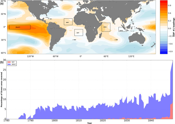
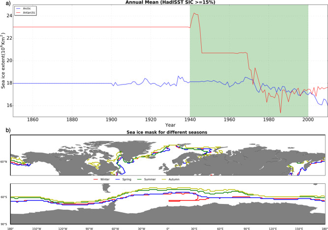
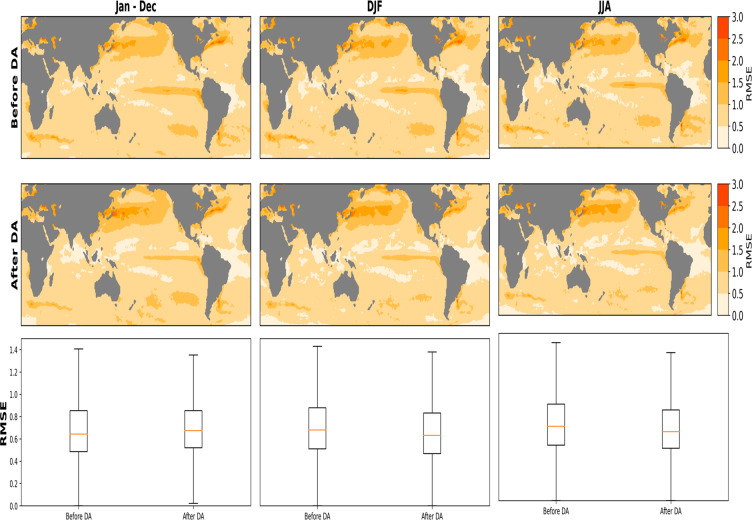
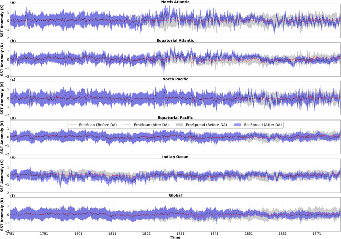
This paper describes a global monthly gridded Sea Surface Temperature (SST) and Sea Ice Concentration (SIC) dataset for the period 1000-1849, which can be used as boundary conditions for atmospheric model simulations. The reconstruction is based on existing coarse-resolution annual temperature ensemble reconstructions, which are then augmented with intra-annual and sub-grid scale variability. The intra-annual component of HadISST.2.0 and oceanic indices estimated from the reconstructed annual mean are used to develop grid-based linear regressions in a monthly stratified approach. Similarly, we reconstruct SIC using analog resampling of HadISST.2.0 SIC (1941-2000), for both hemispheres. Analogs are pooled in four seasons, comprising of 3-months each. The best analogs are selected based on the correlation between each member of the reconstructed SST and its target. For the period 1780 to 1849, We assimilate historical observations of SST and night-time marine air temperature from the ICOADS dataset into our reconstruction using an offline Ensemble Kalman Filter approach. The resulting dataset is physically consistent with information from models, proxies, and observations.

Fig. 1

Schematic diagram, showing sequence of steps involved in reconstructing historical SST and SIC.

Fig. 2

Oceanic indices and coverage of marine observations. (a) The spatial pattern of the first empirical orthogonal function mode (with 30.16% explained variance) of annual SST (K) reconstructed using the analog method by Neukom et al. (2019), calculated over 123 years (1880–2010). The polygons show regions from which we calculate climatic indices. It is important to note that extratropical variability in our reconstruction is always accounted for by tropical variability and its associated teleconnections. (b) Percentage of ocean area covered by marine observations (calculated on 1° × 1° grid boxes) utilized in this study, NMAT (blue) and SST (red) in the assimilation period.

Fig. 3

Zonally averaged partial regression coefficients showing latitudinal variations of SST anomaly (K) for all calendar months. Shown are (a) Nino3.4, which shows seasonal phase-locking of ENSO in the Tropical region; (b) DMI, which develops relative to the annual cycle during the boreal summer month (JJA) and peaks during fall (SON); and (c) TASI, showing the signature of seasonality with warm and cold peaks from January to June and July to December, respectively.

Fig. 4

Pooling and selection of best sea ice analogs. (a) The annual mean sea ice extent as estimated from HadISST SIC for the Arctic (blue) and Antarctic (red). The green shaded area shows the timestamp where analogs are pooled on a seasonal basis, while (b) show regions masked (polewards from different lines) before selecting the best sea ice analog for both Northern and Southern hemispheres.

Fig. 5

Comparison between PaleoSST and HadISST in an overlapping period (1850–1879). (a) Spatial correlation between both data sets before the implementing Data Assimilation (DA) scheme, while (b) shows the same but after DA. (c) and (d) shows the spatial distribution of the root mean square error (K) before and after DA, respectively. (e) The ratio of standard deviation averaged over all calendar months between PaleoSST and IT before DA while (f) shows the same but after DA. Lastly, (g and f) show the MSESS before and after DA, respectively.

Fig. 6

Spatial correlation between the ensemble mean PaleoSST and HadISST in an overlapping period (1850–1879). The first row shows the correlation before implementing Data Assimilation (DA) on Annual (Jan–Dec), boreal winter DJF and boreal summer JJA timescales. The middle row shows the correlation after DA on annual and seasonal timescales (DJF and JJA). The last row summarizes the annual and seasonal spatial correlation over the same overlapping period.

Fig. 7

Root Mean Squared Error (RMSE) ensemble mean between PaleoSST and HadISST in an overlapping period (1850–1879). The first row shows the RMSE before Data Assimilation (DA) scheme, on Annual (Jan–Dec), boreal winter DJF and boreal summer JJA timescales. The middle row shows the RMSE after DA on annual and seasonal timescales (DJF and JJA). The last row summarizes the annual and seasonal RMSE over the same overlapping period.

Fig. 8

Mean Squared Error Skill Score (MSESS) ensemble mean between PaleoSST and HadISST in an overlapping period (1850–1879). The first row shows the MSESS before Data Assimilation (DA) scheme, on Annual (Jan–Dec), boreal winter DJF and boreal summer JJA timescales. The middle row shows the MSESS after DA on annual and seasonal timescales (DJF and JJA). The last row summarizes the annual and seasonal MSESS over the same overlapping period.

Fig. 9

Ensemble spread (EnsSpread) ratio between reconstructed SSTs before and after data assimilation (After DA/Before DA) calculated over the whole assimilation period (1781–1879).

Fig. 10

The temporal evolution of ensemble spread (EnsSpread) before and after DA, calculated as mean anomalies over the entire assimilation period (1781–1879) for selected ocean regions. Shown are (a) North Atlantic (291°–358°, 21.5°–65.5° N) (b) Equatorial Atlantic (291°–358°, −22.5–21.5° N) (c) North Pacific (120°–238°, 21.5°–55.5° N) (d) Equatorial Pacific (120°–238°, −22.5°–21.5° N) (e) Indian Ocean (34.5°–108°, −22.5°–14.5° N) and (f) Global. The grey shade and red line show the EnsSpread and ensemble mean (EnsMean) before DA, while the blue shade and black dashed line depicts the EnsSpread and EnsMean after DA, respectively.

Fig. 11

Average intra-annual standard deviation (K). (a) PaleoSST, (b) SODAsi3.0 SST and (c) augmented version^, of Mann et al., (2009) SST, in an overlapping period (1820–1849).

Fig. 12

Variability in reconstructed sea ice concentration. (a) Annual mean sea ice extent (1000–1849), showing inter-annual variability in a single ensemble member for the Arctic (blue) and Antarctic (red). (b) Arctic sea ice extent for a specific month (June) across the reconstruction period.

References

1. Kennedy JJ, Rayner NA, Atkinson CP, Killick RE. An ensemble data set of sea surface temperature change from 1850: The Met Office Hadley Centre HadSST.4.0.0.0 data set. Journal of Geophysical Research: Atmospheres. 2019;124:7719–7763.
1. Rayner NA, et al. Global analyses of sea surface temperature, sea ice, and night marine air temperature since the late nineteenth century. Journal of Geophysical Research: Atmospheres. 2003;108:D14. doi: 10.1029/2002JD002670. - DOI
1. Giese BS, Seidel HF, Compo GP, Sardeshmukh PD. An ensemble of ocean reanalyses for 1815–2013 with sparse observational input. J. Geophys. Res. Oceans. 2016;121:6891–6910. doi: 10.1002/2016JC012079. - DOI
1. Mann ME, et al. Global signatures and dynamical origins of the Little Ice Age and Medieval Climate Anomaly. Science. 2009;326:1256–1260. doi: 10.1126/science.1177303. - DOI - PubMed
1. Tardif R, et al. Last Millennium Reanalysis with an expanded proxy database and seasonal proxy modeling. Clim. Past. 2019;15:1251–1273. doi: 10.5194/cp-15-1251-2019. - DOI