Hierarchical Censored Bayesian Analysis of Visual Field Progression

Abstract

Purpose: To develop a Bayesian model (BM) for visual field (VF) progression accounting for the hierarchical, censored and heteroskedastic nature of the data.

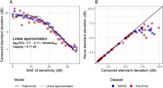
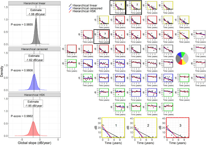
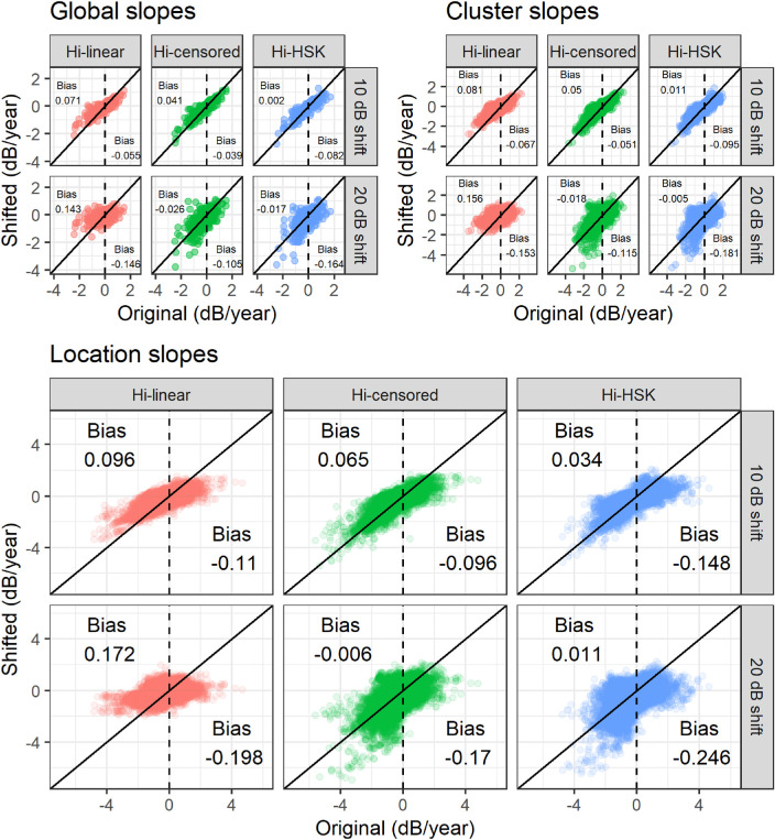
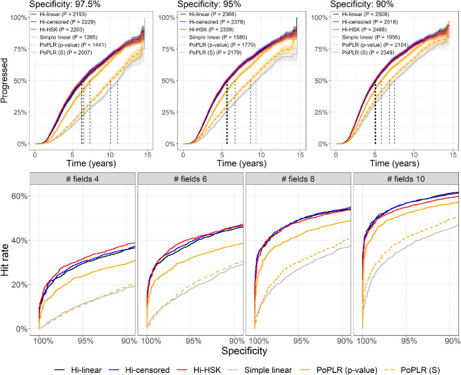
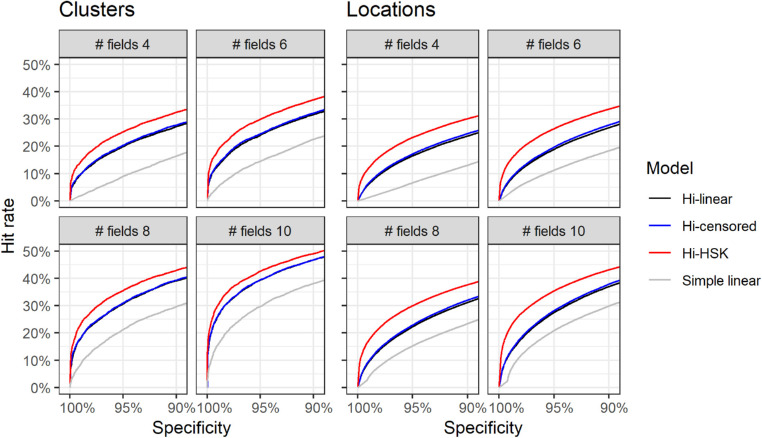
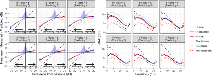
Methods: Three versions of a hierarchical BM were developed: a simple linear (Hi-linear); censored at 0 dB (Hi-censored); heteroskedastic censored (Hi-HSK). For the latter, we modeled the test variability according to VF sensitivity using a large test-retest cohort (1396 VFs, 146 eyes with glaucoma). We analyzed a large cohort of 44,371 VF tests from 3352 eyes from five glaucoma clinics. We quantified the bias in the estimated rate-of-progression, the detection of progression (Hit-rate [HR]), the median time-to-progression and the prediction error of future observations (mean absolute error [MAE]). HR and time-to-progression were compared at matched false-positive-rate (FPR), quantified using permutations of a separate test-retest cohort (360 tests, 30 eyes with glaucoma). BMs were compared to simple linear regression and Permutation-Analyses-of Pointwise-Linear-Regression. Differences in time-to-progression were tested using survival analysis.

Results: Censored models showed the smallest bias in the rate-of-progression. The three BMs performed very similarly in terms of HR and time-to-progression and always better than the other methods. The average reduction in time-to-progression was 37% with the BMs (P < 0.001) at 5% FPR. MAE for prediction was very similar among methods.

Conclusions: Bayesian hierarchical models improved the detection of VF progression. Accounting for censoring improves the precision of the estimates, but minimal effect is provided by accounting for heteroskedasticity.

Translational relevance: These results are relevant for quantification of VF progression in practice and for clinical trials.

Figure 1.

Panel A shows how the censored standard deviation for test-retest variability changes at different sensitivity levels and the corresponding predictions from the polynomial model and the bi-linear approximation. Panel B shows the comparison between naïve and censored standard deviation. Data-points are reported for both test-retest datasets but the models were only based on the RAPID dataset.

Figure 2.

The panel on the right shows an example of a visual field series, fitted with the different hierarchical models. In the superior hemifield, it is evident how the censored models are less affected by the floor effect. The borders of the subplots are color-coded to indicate the cluster corresponding to different optic nerve head sectors (circular schematic in the blind-spot locations). The panels on the left show the posterior distribution for the global slope from the for the same field series, with the corresponding P-score, equivalent to the shaded area under the curve. The censored models produce less positively biased distributions, but with larger variance, reflecting the fact that censored sensitivity values only provide partial information. Hi = Hierarchical; HSK = Heteroskedastic.

Figure 3.

Comparison between the slopes estimated by the different models in the artificially shifted series and the original series. Note that the artificial series are shifted downward towards lower values. The censored models are less affected by a positive bias on the negative slopes compare to the Hi-linear model. The average bias for the negative and for the positive slopes is reported in the figure. Hi = Hierarchical; HSK = Heteroskedastic.

Figure 4.

The top panels present the Kaplan-Meier curves for all tested methods at different specificity levels. P in the legends indicate the number of eyes that progressed with each method. The vertical dashed lines indicated the median time to progression (not color coded). The bottom panels show curves of the hit-rate at different specificity levels for all the progression methods tested with the series truncated at different lengths. Hi = Hierarchical; HSK = Heteroskedastic.

Figure 5.

Curves of hit-rates at different specificities for individual visual field clusters and locations at different lengths of the series. Note that a “hit” is progression in any cluster, or location, and the percentages are calculated over the total number of clusters (N = 20,112) and locations (N = 174,304). Hi = Hierarchical; HSK = Heteroskedastic.

Figure 6.

Average error for pointwise prediction stratified by difference from baseline (left panel) and mean absolute error stratified by baseline VF sensitivity (right panel) for the different hierarchical models and the pointwise linear regression. The density profile in the left panels represent the actual distribution of differences observed in the data. The diagonal dashed line represents the error resulting from predicting no change. Hi = Hierarchical; HSK = Heteroskedastic.

References

1. Garway-Heath DF, Poinoosawmy D, Fitzke FW, Hithings RA.. Mapping the visual field to the optic disc in normal tension glaucoma eyes. Ophthalmology. 2000; 107: 1809–1815. - PubMed
1. Jansonius NM, Nevalainen J, Selig B, et al. .. A mathematical description of nerve fiber bundle trajectories and their variability in the human retina. Vision Res. 2009; 49: 2157–2163. - PMC - PubMed
1. Denniss J, McKendrick AM, Turpin A.. An anatomically customizable computational model relating the visual field to the optic nerve head in individual eyes. Invest Ophthalmol Vis Sci. 2012; 53: 6981–6990. - PubMed
1. Henson DB, Chaudry S, Artes PH, Faragher EB, Ansons A.. Response variability in the visual field: comparison of optic neuritis, glaucoma, ocular hypertension, and normal eyes. Invest Ophthalmol Vis Sci. 2000; 41: 417–421. - PubMed
1. Chauhan BC, Tompkins JD, LeBlanc RP, McCormick TA.. Characteristics of frequency-of-seeing curves in normal subjects, patients with suspected glaucoma, and patients with glaucoma. Invest Ophthalmol Vis Sci. 1993; 34: 3534–3540. - PubMed