Spatially resolved cell atlas of the mouse primary motor cortex by MERFISH

Abstract

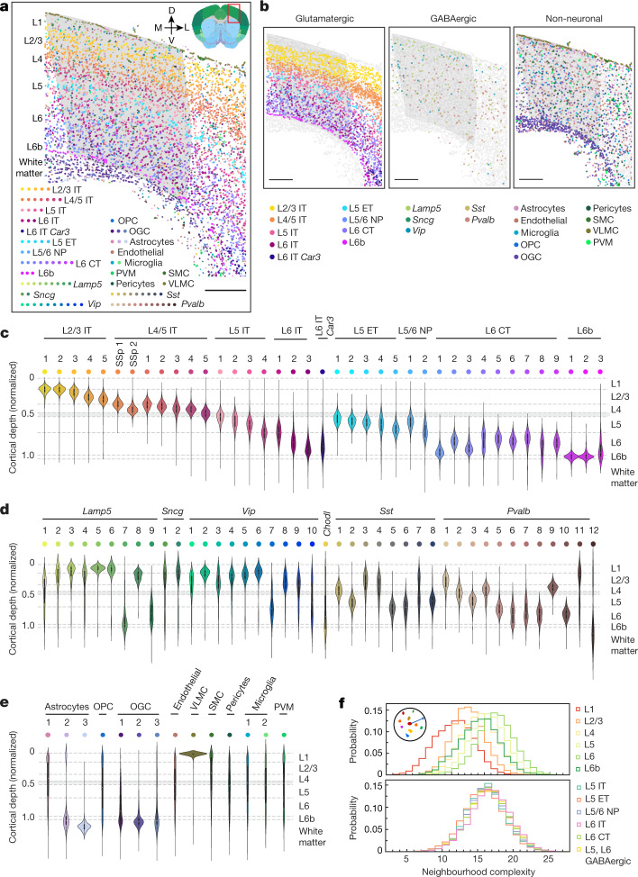
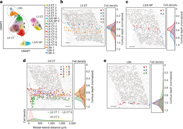
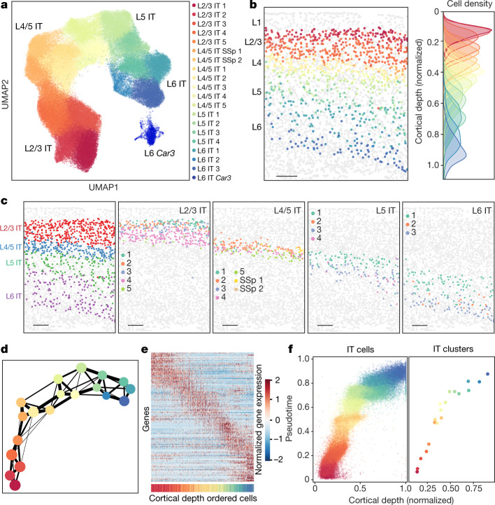
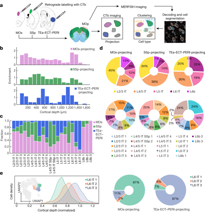
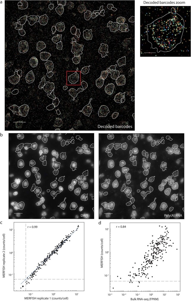
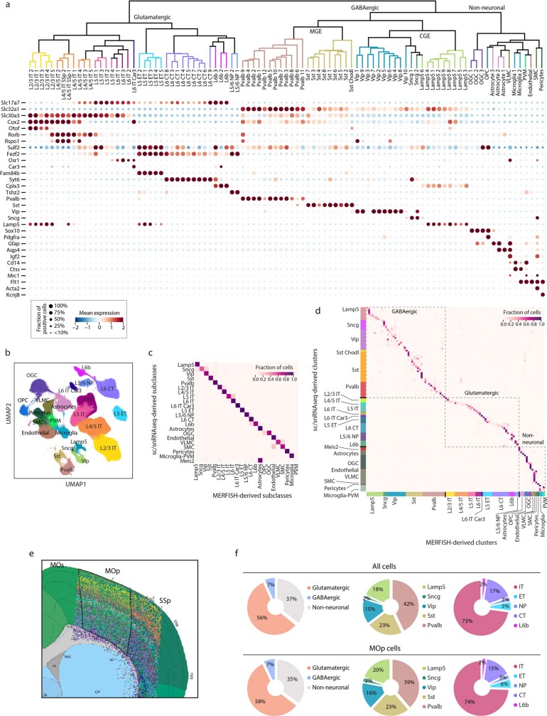
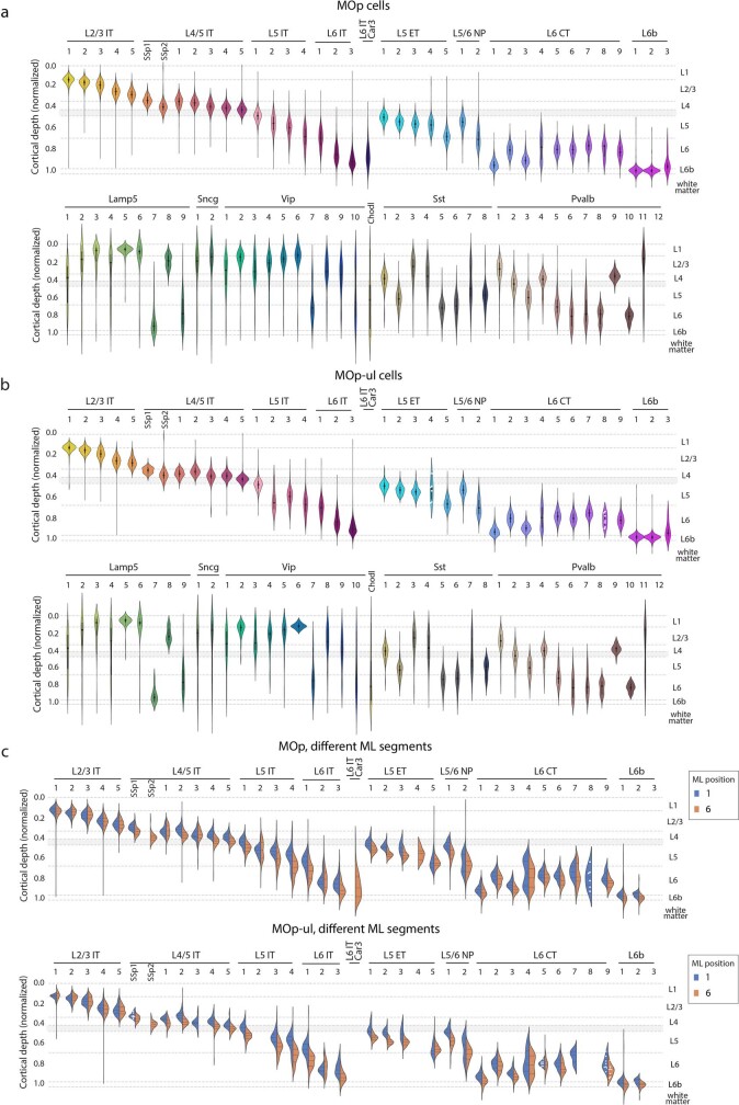
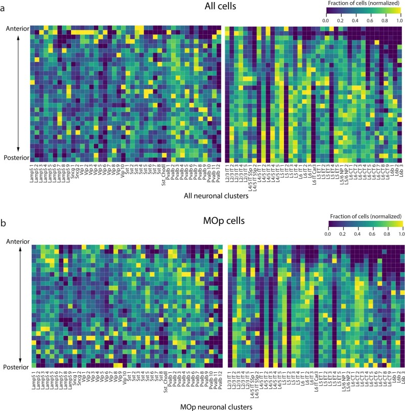
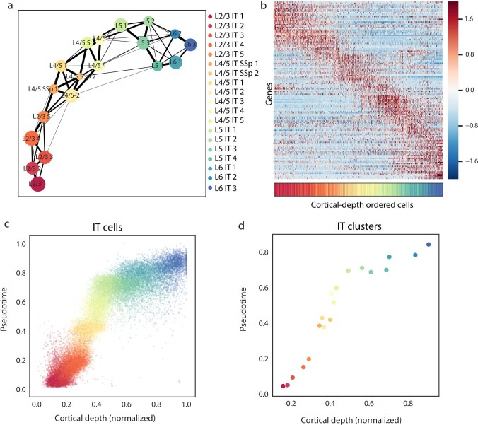
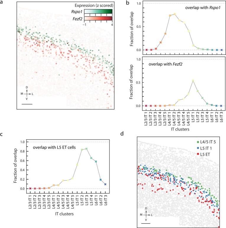
A mammalian brain is composed of numerous cell types organized in an intricate manner to form functional neural circuits. Single-cell RNA sequencing allows systematic identification of cell types based on their gene expression profiles and has revealed many distinct cell populations in the brain^1,2. Single-cell epigenomic profiling^3,4 further provides information on gene-regulatory signatures of different cell types. Understanding how different cell types contribute to brain function, however, requires knowledge of their spatial organization and connectivity, which is not preserved in sequencing-based methods that involve cell dissociation. Here we used a single-cell transcriptome-imaging method, multiplexed error-robust fluorescence in situ hybridization (MERFISH)⁵, to generate a molecularly defined and spatially resolved cell atlas of the mouse primary motor cortex. We profiled approximately 300,000 cells in the mouse primary motor cortex and its adjacent areas, identified 95 neuronal and non-neuronal cell clusters, and revealed a complex spatial map in which not only excitatory but also most inhibitory neuronal clusters adopted laminar organizations. Intratelencephalic neurons formed a largely continuous gradient along the cortical depth axis, in which the gene expression of individual cells correlated with their cortical depths. Furthermore, we integrated MERFISH with retrograde labelling to probe projection targets of neurons of the mouse primary motor cortex and found that their cortical projections formed a complex network in which individual neuronal clusters project to multiple target regions and individual target regions receive inputs from multiple neuronal clusters.

Fig. 1. Spatial organization of cells in the MOp and adjacent areas.

a, Spatial map of the cell clusters in a coronal slice (Bregma approximately +0.9). Cells are coloured by their cluster identities. The MOp region, determined based on the Allen CCF v3, is shaded in grey. The inset shows the brain region annotations in the Allen CCF v3 (http://atlas.brain-map.org/; credit: Allen Institute). D, dorsal; L, lateral; M, medial; OGC, oligodendrocyte; OPC, oligodendrocyte precursor cell; PVM, perivascular macrophage; SMC, smooth muscle cell; V, ventral; VLMC, vascular leptomeningeal cell. Scale bar, 400 μm. b, Spatial map of the cell subclasses in glutamatergic (left), GABAergic (middle) and non-neuronal (right) cells in the same slice as in a. Cells are shown as circles, with indicated cells coloured by subclasses and others in grey. Scale bars, 400 μm. c–e, The cortical depth distributions of the glutamatergic (c), GABAergic (d) and non-neuronal (e) clusters for the entire imaged region including the MOp and adjacent areas shown in the violin plots. The cortical depth of a cell is normalized by the cortical thickness in each slice, with 0 representing the cortical surface and 1 representing the median depth of the L6b cells. The dashed lines mark the layer boundaries, and the grey area marks an uncertainty range for the upper boundary of L5 (Methods). In the violin plots, the centre dot represents the median, the thick black bar represents the interquartile range, and the edges define minima and maxima. f, Probability distributions of the neighbourhood complexity of cells in each cortical layer (top) and in different cell subclasses in L5 and L6 (bottom). The neighbourhood complexity of a cell is defined as the number of different cell clusters present within a neighbourhood of 100 μm in radius surrounding the given cell.

Fig. 2. Spatial organization of the L5 ET, L5/6 NP, L6 CT and L6b neurons.

a, Uniform manifold approximation and projection (UMAP) of the L5 ET, L5/6 NP, L6 CT and L6b neurons coloured by the cluster identity. b, Spatial map of L5 ET cell clusters in a coronal slice (Bregma approximately +0.8). L5 ET cells are coloured, and other cells in the MOp are shown in dark grey to highlight the MOp region, whereas other cells outside the MOp are shown in light grey. Normalized cortical depth distributions of the cells of each L5 ET cluster are shown in the right panel and presented in the form of the Kernel density of the distribution histograms. c, Spatial map of L5/6 NP cell clusters in a coronal slice (Bregma approximately +0.4) and the normalized cortical depth distributions of these clusters, as in b. d, Spatial map of the L6 CT cell clusters in a coronal slice (Bregma approximately +0.3) and the normalized cortical depth distributions of these clusters, as in b. The medial–lateral distribution for clusters 1, 5 and 8 are also shown at the bottom. The medial–lateral distribution is calculated in the coronal slices in which cluster 8 is present. e, Spatial map of the L6b clusters in a coronal slice (Bregma approximately +0.4) and the normalized cortical depth distributions of these clusters, as in b. Scale bars, 200 μm (b–e).

Fig. 3. Correlated gene expression and spatial gradients across IT neurons.

Analyses of IT neurons in the entire imaged region are shown here and the corresponding analyses for the MOp are shown in Extended Data Figs. 8, 9. a, UMAP of the IT clusters coloured by the cluster identity. b, Spatial map of IT neurons in a coronal slice (Bregma approximately +1.0). The IT neurons are coloured by their cluster identity as in a, and all other cells are in grey (left). Scale bar, 200 μm. The cortical depth distributions of individual IT clusters are also shown (right). c, Spatial maps of the L2/3, L4/5, L5 and L6 IT subclasses (left panel) and individual clusters in each subclass (four right panels) in the same coronal slice as in b. Scale bars, 200 μm. d, The degree of connectivity between clusters in a k-nearest neighbour graph for the IT clusters, with each cluster represented as a node coloured as in a, and the weighted edges between nodes representing their connectivity. Edges with weights below 0.1 are not shown. e, Normalized expression of differentially expressed genes of all IT neurons across cortical depth. Here, differentially expressed genes refer to genes of which the expression varied substantially with cortical depth (Methods). Individual IT neurons were sorted in the order of ascending cortical depth and the genes were sorted by the cortical depth at which they exhibit maximal expression. The coloured bar at the bottom indicates the cluster identity of the cell, coloured as in a. f, Scatter plot of the pseudotime versus normalized cortical depth for individual IT neurons (left) and individual IT clusters (right) in the L2/3, L4/5, L5 and L6 IT subclasses coloured by the cell clusters, as in a.

Fig. 4. Projection patterns of IT neurons determined by integration of MERFISH with retrograde labelling.

a, Workflow integrating retrograde labelling and MERFISH. CTb-AlexaFluor647, CTb-AlexaFluor555 and CTb-AlexaFluor488 were injected into the MOs, SSp and TEa–ECT–PERI regions, respectively. The coronal slices containing the MOp on the ipsilateral side of these targets were imaged for both the retrograde CTb labels and the MERFISH gene panel. The mouse brain CCF image shown on the left is from the Allen Brain Atlas (http://atlas.brain-map.org/; credit: Allen Institute). Endo, endothelial cell. b, Enrichment of MOs-projecting, SSp-projecting and TEa–ECT–PERI-projecting cells at different cortical depths. Enrichment is defined as the fraction of relevant CTb-positive cells divided by the fraction of all IT and L6b cells in the same bin. c, Fractions of MOs-projecting, SSP-projecting and TEa–ECT–PERI-projecting cells in each cell cluster among all CTb-positive, single-projecting cells in the cluster. d, Pie charts showing the proportions of MOs-projecting (left), SSp-projecting (middle) and TEa–ECT–PERI-projecting (right) cells belonging to each cell subclass (top) and cluster (bottom; only top 10 clusters shown). The mean fractions are shown and the 95% confidence intervals are less than 0.7%. e, Projection specificity of the molecularly and spatially similar L6 IT clusters. The cortical depth distributions of the L6 IT 1–3 clusters and the UMAP (inset) are displayed, with L6 IT 1–3 neurons shown in colours and other IT neurons shown in grey (left). Pie charts showing the relative proportions of MOs-projecting and TEa–ECT–PERI-projecting L6 IT neurons that belong to each of the three clusters are also displayed (right). The mean fractions are shown and the 95% confidence intervals are less than 1%.

Extended Data Fig. 1. RNA identification and cell segmentation of MERFISH images, replicate reproducibility of MERFISH data, and correlation between MERFISH and bulk RNA-seq results.

a, Decoded MERFISH image of a single field-of-view, shown as a maximum intensity projection across all seven z-planes. In these experiments, we assigned 22-bit Hamming Distance 4, Hamming Weigh 4 barcodes capable of error detection and correction to individual RNA species, and the 22 bits were imaged in 11 rounds of hybridization with two-colour imaging per round. The decoded image shows all pixels that belonged to detected correct barcodes. The pixels were coloured based on their assigned barcodes and the intensity of each pixel was scaled based on the L2-norm of its signal intensity across all bits. Segmented cell boundaries are shown in white. The boxed region of the image is shown at a greater magnification (right). Scale bars, 20 μm (left) and 5 μm (right). b, DAPI (left) and poly(A) RNA (right) images for the same field of view as in a, with the central z-plane (z = 4.5 μm) shown. These images are used to define the boundaries of each cell, shown in white. Scale bars, 20 μm. a and b are representative images of more than 5,000 fields of view from two replicate animals. c, Scatterplot of the average copy number per cell of individual genes measured by MERFISH for the two replicate animals. The blue solid line indicates equality. The grey dashed lines indicate the average counts per cell of the blank barcodes (that is, valid barcodes that were not assigned to any RNA), which provides an estimate of the false-positive rate. The Pearson correlation coefficient is r = 0.99. d, Scatterplot of the average copy number per cell of individual genes determined by MERFISH versus expression level determined by bulk RNA-seq. The dashed line is as defined in c. The Pearson correlation coefficient is r = 0.84.

Extended Data Fig. 2. Cell-type profiling by MERFISH, registration of MERFISH images to Common Coordinate Framework and the composition of cells.

a, Dendrogram showing the hierarchical relationship among the 39 glutamatergic, 42 GABAergic, and 14 non-neuronal clusters identified by MERFISH, constructed based on the z-scored cluster expression profiles and coloured by the subclass that each cluster belongs to (top). Expression of markers genes for the subclasses are also displayed (bottom). b, UMAP of cells measured by MERFISH coloured based on the subclasses of cells. c, Correspondence between the subclasses of cells determined by MERFISH and the subclasses determined by scRNA-seq and snRNA-seq datasets generated in a companion study. A neural-net classifier was used to predict a MERFISH cluster label for each cell in the snRNA-seq 10x v3 B dataset. The fraction of cells from any given subclass identified by scRNA-seq and snRNA-seq that was predicted to have each MERFISH subclass label was plotted. d, Correspondence between clusters identified by MERFISH and by scRNA-seq and snRNA-seq. As in c, but with the fraction of cells from any given cluster identified by scRNA-seq and snRNA-seq that was predicted to have each MERFISH cluster label plotted. Each row or column corresponds to a cluster and the coloured bars on the left and bottom mark the subclasses. e, An example MERFISH-derived cell-type spatial map overlaid on the Allen CCF v3 with cells coloured by their cluster identities as in Fig. 1a. The CCF v3 image is from the Allen Brain Atlas (http://atlas.brain-map.org/; credit: Allen Institute). The boundaries of the MOp are shown in black. We note that the MOp–MOs and MOp–SSp borders, as well as all other cortical area borders in the Allen CCF v3, are largely perpendicular to the cortical surface in the 3D space. The reason that they do not always appear perpendicular to the cortical surface line in the coronal sections, as shown here, is because the coronal sections themselves are not always perpendicular to the cortical surface (see more details about this effect at: https://community.brain-map.org/t/ccfv3-highlights-tilting-at-the-cortex/1000; credit: Allen Institute). f, Top: fractions of cells in the entire imaged region that belong to each of the three major cell classes (glutamatergic, GABAergic and non-neuronal) (left). Fractions of GABAergic cells in the entire imaged region that belong to each of the GABAergic subclasses (middle). Fractions of glutamatergic cells in the entire imaged region that belong to each of the glutamatergic subclasses (right). The mean fractions are shown and the 95% confidence intervals are less than 0.3%. Bottom: same as the top panel but for cells in the MOp. The mean fractions are shown and the 95% confidence intervals are less than 0.4%.

Extended Data Fig. 3. Cortical depth distributions of neuronal cell clusters in the MOp and an approximate MOp upper limb region.

a, b, As in Fig. 1c, d but for glutamatergic and GABAergic clusters in the MOp (a) and an approximate MOp upper limb (MOp-ul) region (b). We selected the region between Bregma 0 and +1.0 within the MOp as an approximation for the MOp-ul region based on previous literature and a companion paper. This region is considered as the primary part of the MOp-ul because it contains the densest pyramidal neurons that directly project to the intermediate horn and ventral horn of the cervical spinal cord and, in the meantime, shows minimal projection to the lower limb. In the violin plots, the black dot represents the median, the thick black bar represents the interquartile range, and the edges define minima and maxima. c, Effect of the layer-thickness variations along the medial–lateral (ML) direction on the cortical depth distributions of the neuronal clusters. Top: we divided the MOp into six segments along the ML direction, each covering a narrow ML range such that the layer-thickness variations within each segment are negligible. We then determined the cortical depth distributions of the neuronal clusters in each of the six ML segments and display those for the most medial (blue; ML position 1) and most lateral (orange; ML position 6) segments. Most of the clusters showed only a modest difference in their cortical depth distributions between different ML segments, with a small number of exceptions (such as L4/5 IT SSp 1 and 2, L5 ET 4, L6 CT 8 and L6 IT Car 3). These exceptions showed large differences due to the region-dependent presence of these clusters. Only the distributions of the glutamatergic clusters are shown here because the relatively low abundance of the GABAergic neurons makes the comparison of their distributions in different ML segments statistically less sound. Bottom: as in the top panel but for glutamatergic clusters in the approximate MOp-ul region as defined in b. In the violin plots in c, the centre dashed line represents the median, the other two dashed lines represent the interquartile range, and the edges define minima and maxima. For all violin plots in a–c, the clusters with cell numbers of five or fewer are not shown, and the clusters with cell numbers of ten or fewer (but more than five) are shown with individual data points as white dots.

Extended Data Fig. 4. Anterior–posterior distribution of neuronal clusters.

a, Heatmap quantifying the anterior–posterior distribution of the neuronal clusters in the entire imaged region including the MOp and its adjacent areas. Slices were arranged from anterior-most to posterior-most based on their Bregma coordinates (Bregma +2.5 to −0.8). For each cluster, the fraction of cells found in each slice was determined and normalized to the maximum across all slices. b, As in a but for the neurons within the MOp.

Extended Data Fig. 5. Neighbourhood complexity of individual cells belonging to different subclasses.

The neighbourhood complexity of a cell is defined as in Fig. 1f. A normalized histogram of the neighbourhood complexity for all cells from a given subclass is shown for each cell subclass.

Extended Data Fig. 6. Additional analyses of the L5 ET, L5/6 NP, L6 CT and L6b clusters.

a, Correspondence between the L5 ET, L5/6 NP, L6 CT and L6b clusters determined by MERFISH and those identified by scRNA-seq and snRNA-seq. b, Correspondence between the L5 ET, L6 CT, L5/6 NP and L6b clusters determined by MERFISH and those identified by integrated analysis of scRNA-seq, snRNA-seq, snATAC-seq and snmC-Seq datasets using SingleCellFusion. The classifier approach used in a and b to determine the correspondence is as described in Extended Data Fig. 2c. c, Left: a coronal slice (Bregma approximately +0.7) highlighting the L5 ET cells coloured by cell clusters in the MOp and the neighbouring SSp region. Cells other than the L5 ET cells are shown in dark grey in the MOp to highlight the MOp region, and cells other than the L5 ET cells outside the MOp are shown in light grey. Scale bars, 200 μm. Right: comparison of the abundance of L5 ET 5 neurons in the MOp and SSp. The fraction of L5 ET 5 cells with respect to the total cell number detected in the MOp or SSp are shown. n = 2 replicate animals, with individual data points from each animal shown.

Extended Data Fig. 7. Correspondence between the MERFISH IT clusters and the IT clusters determined by scRNA-seq and snRNA-seq analysis and by integrated analysis, and spatial distributions of L6 IT Car3 and L4/5 IT SSp 1 and 2 clusters.

a, Correspondence between the IT clusters identified by MERFISH and those identified by scRNA-seq and snRNA-seq. b, Correspondence between the IT clusters identified by MERFISH and those identified by the integrated clustering analysis of scRNA-seq, snRNA-seq, snATAC-seq and snmC-seq using SingleCellFusion. The correspondence in a and b is determined using a classifier approach as described in Extended Data Fig. 2c. c, A coronal slice (Bregma approximately +1.1) highlighting the L6 IT Car3 cluster (green). d, A coronal slice (Bregma approximately +0.9) highlighting the L4/5 IT SSp 1 (green) and L4/5 IT SSp 2 (orange) clusters. In both c and d, all other cells within the MOp are coloured in dark grey to highlight the MOp region, and all other cells outside the MOp are shown in light grey. Scale bars, 200 μm (c, d).

Extended Data Fig. 8. Gene expression profiles and cortical depth distributions of IT cell clusters in the MOp.

a, UMAP of the IT clusters for cells in the MOp. b, Cortical depth distributions of IT clusters in the MOp region, with individual IT clusters coloured as in a. c, Cortical depth distributions of IT clusters in different medial–lateral (ML) segments of the MOp region. The IT clusters are coloured as in a. As the variation in layer thicknesses along the ML direction could broaden the cortical depth distributions of the clusters, to assess whether the spatial overlap between different IT clusters could be caused by this effect, we divided the MOp into six segments along the ML direction, each covering a narrow ML range such that the layer-thickness variations within each ML segment are negligible. We then determined the cortical depth distributions of the IT clusters in each of the six ML segments. The spatial overlap between the IT clusters was still observed in each of the six ML segments. d, Cortical depth distributions of IT clusters in different ML segments in the approximate MOp upper limb region (between Bregma 0 and +1.0, as defined in Extended Data Fig. 3b). The spatial overlap between the IT clusters was still observed in each of the six ML segments in this region. Clusters with a low cell number (five or fewer) found in any individual ML segments are not shown.

Extended Data Fig. 9. Correlated gradients in gene expression and cortical depth across IT neurons in the MOp.

a, Same as Fig. 3d, but for IT neurons in the MOp. b, Same as Fig. 3e, but for differentially expressed genes of all IT neurons within the MOp across cortical depth. c, d, Same as Fig. 3f, but for individual IT cells (c) and individual IT clusters (d) in the MOp.

Extended Data Fig. 10. Spatial overlap between individual IT clusters and the L4 marker gene Rspo1, the L5 marker gene Fezf2 and L5 ET cells.

a, A coronal slice (Bregma approximately +1.0) highlighting the IT cells that express Rspo1 (green) and Fezf2 (red). Scale bar, 200 μm. b, Spatial overlap between individual IT clusters and Rspo1 (top) and Fezf2 (bottom). c, Spatial overlap between individual IT clusters and L5 ET cells. d, The same coronal slice as in a, but highlighting the L4/5 IT 5 (green), L5 IT 1 (blue) and L5 ET (red) cells. Scale bar, 200 μm. See Methods (‘Layer boundary assessment’ section) for how the spatial overlap is determined.

References

1. Poulin JF, Tasic B, Hjerling-Leffler J, Trimarchi JM, Awatramani R. Disentangling neural cell diversity using single-cell transcriptomics. Nat. Neurosci. 2016;19:1131–1141. doi: 10.1038/nn.4366. - DOI - PubMed
1. Zeng H, Sanes JR. Neuronal cell-type classification: challenges, opportunities and the path forward. Nat. Rev. Neurosci. 2017;18:530–546. doi: 10.1038/nrn.2017.85. - DOI - PubMed
1. Kelsey G, Stegle O, Reik W. Single-cell epigenomics: recording the past and predicting the future. Science. 2017;358:69–75. doi: 10.1126/science.aan6826. - DOI - PubMed
1. Zhu C, Preissl S, Ren B. Single-cell multimodal omics: the power of many. Nat. Methods. 2020;17:11–14. doi: 10.1038/s41592-019-0691-5. - DOI - PubMed
1. Chen KH, Boettiger AN, Moffitt JR, Wang S, Zhuang X. Spatially resolved, highly multiplexed RNA profiling in single cells. Science. 2015;348:aaa6090. doi: 10.1126/science.aaa6090. - DOI - PMC - PubMed
Publication types