Cellular anatomy of the mouse primary motor cortex

Abstract

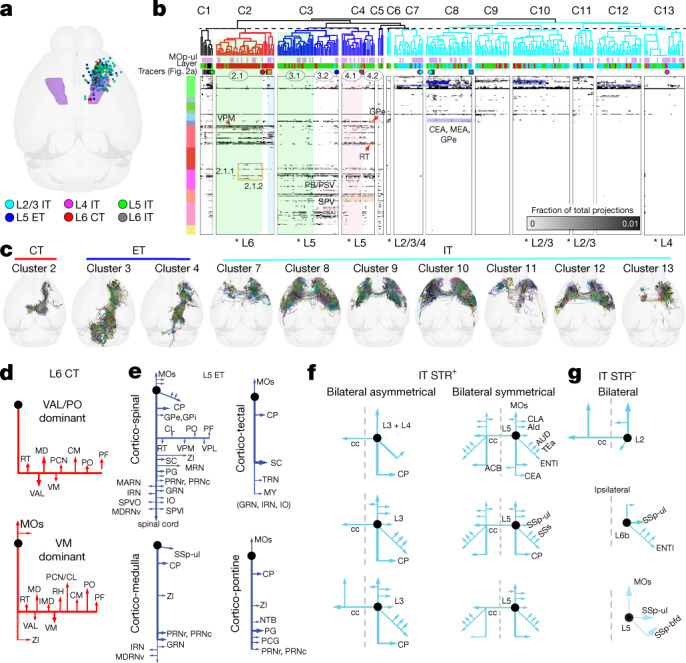
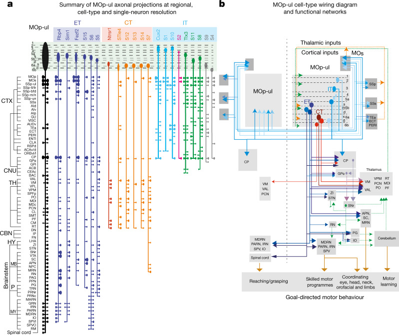
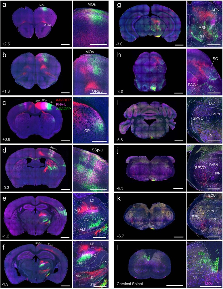
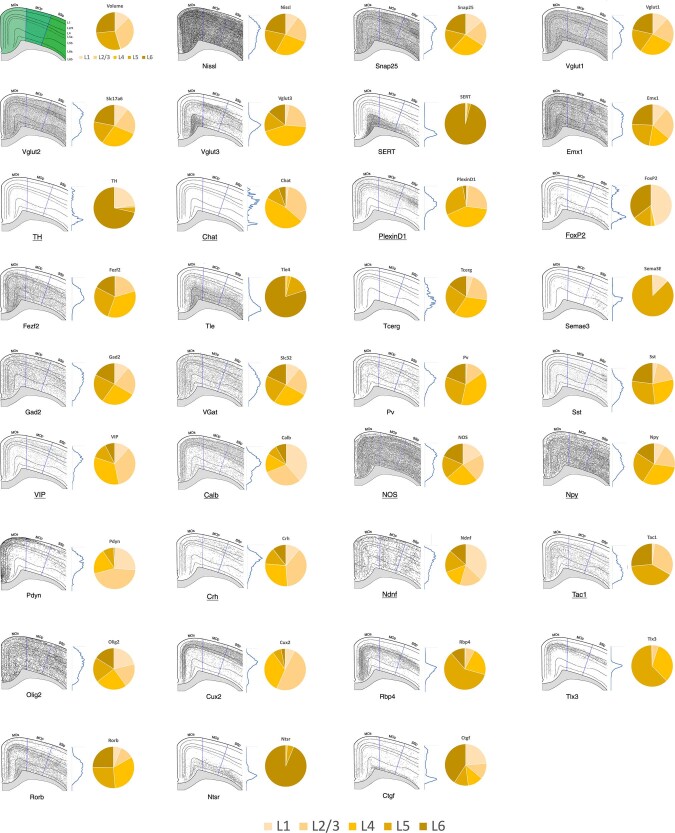
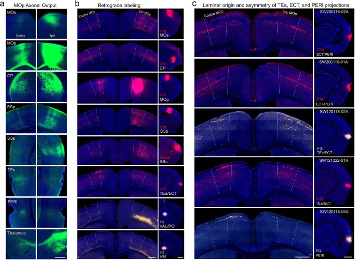
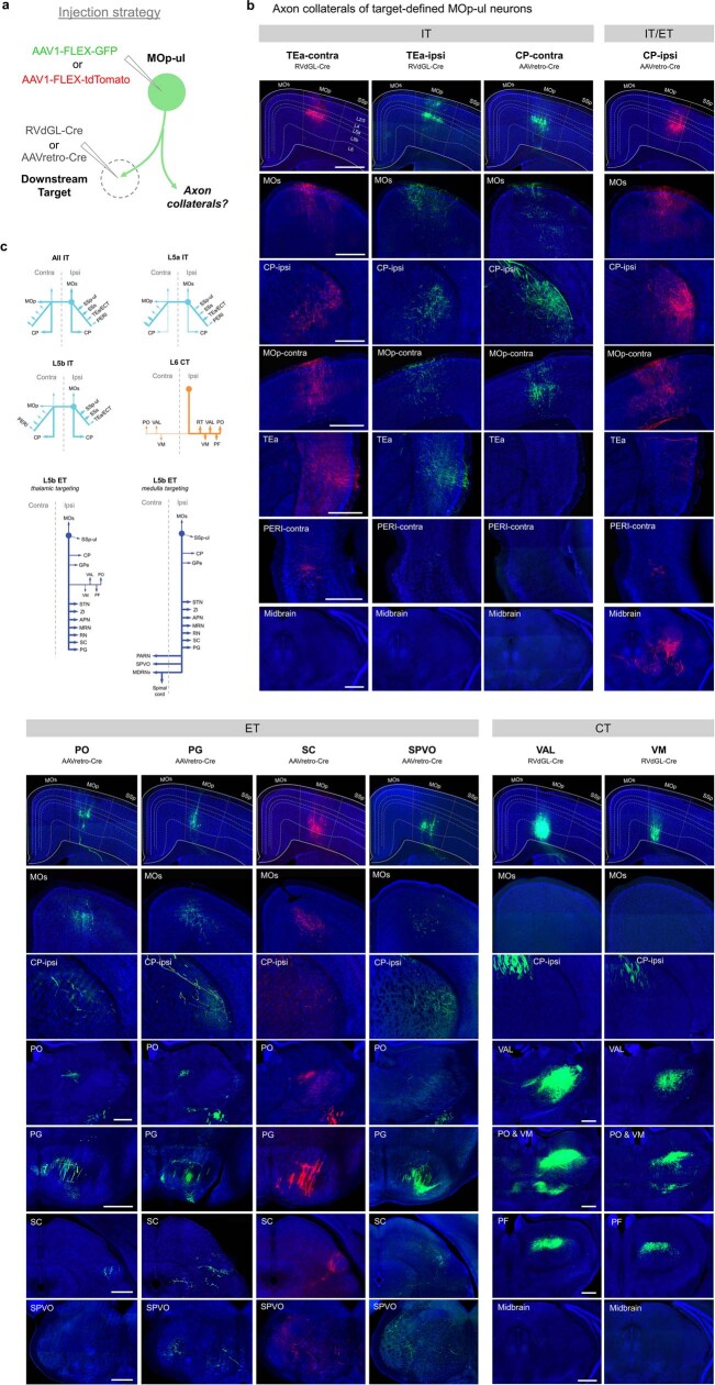
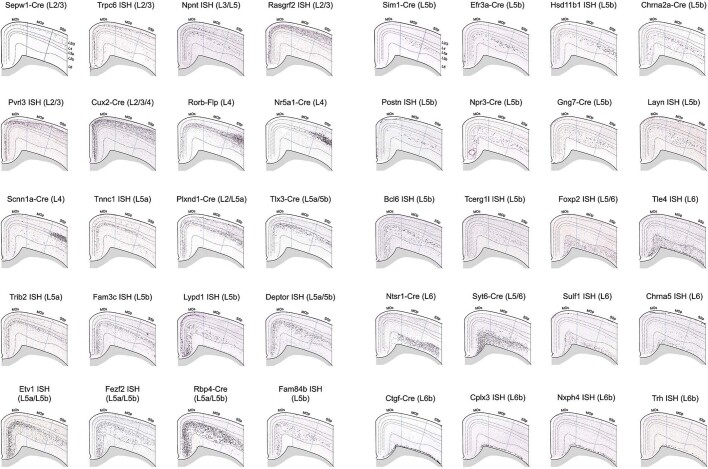
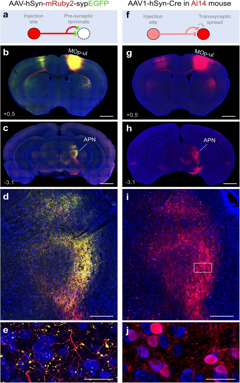
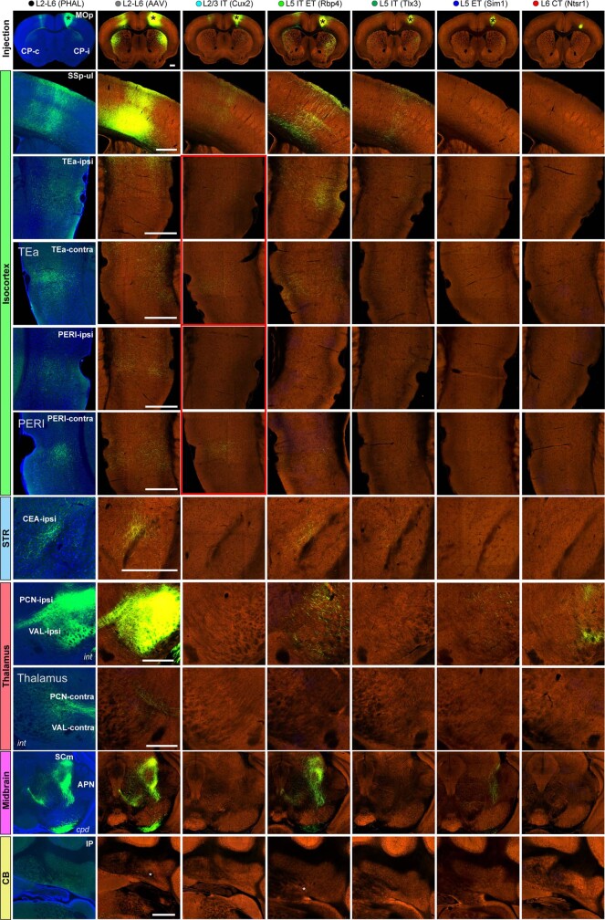
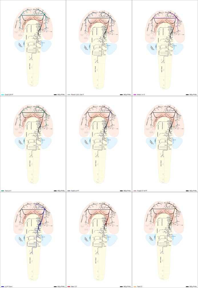
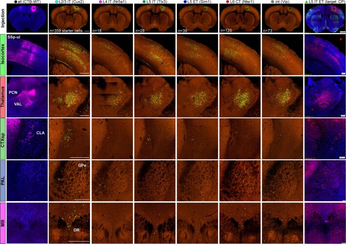
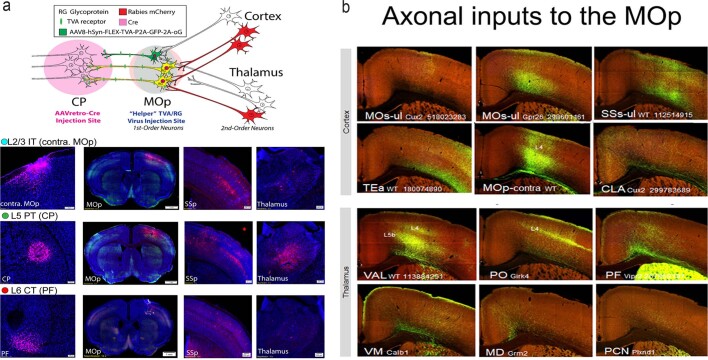
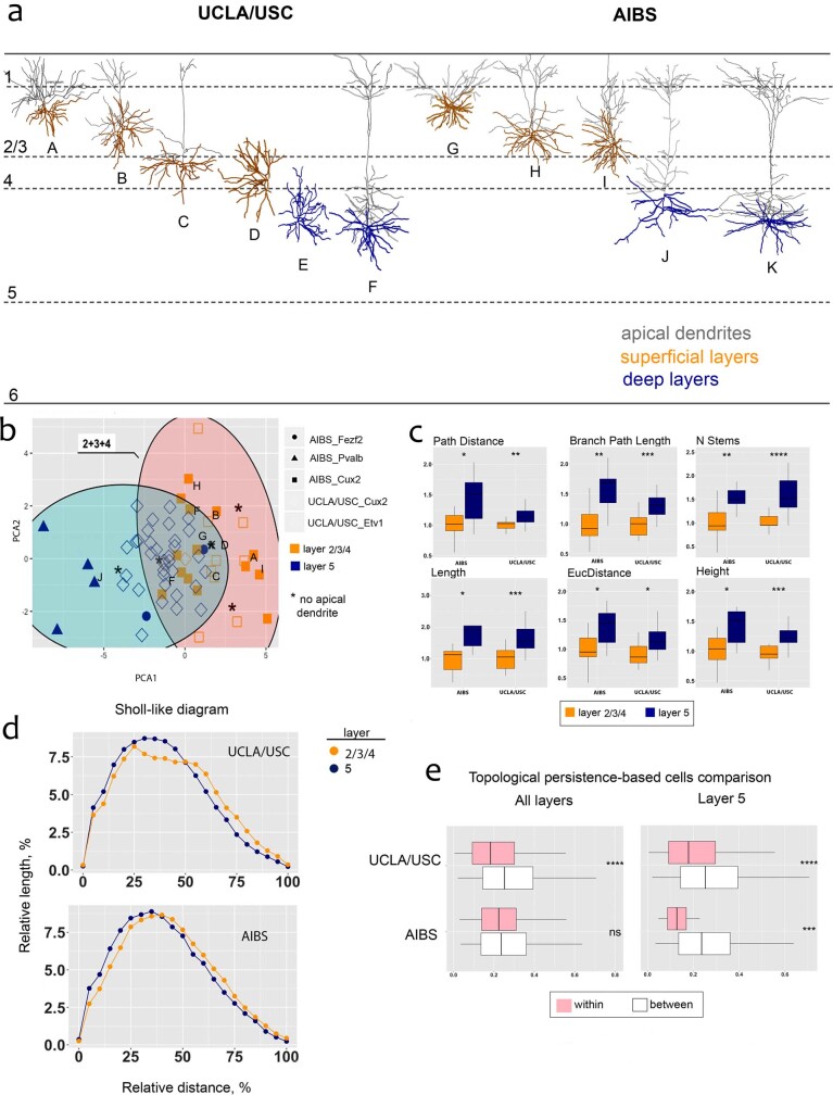
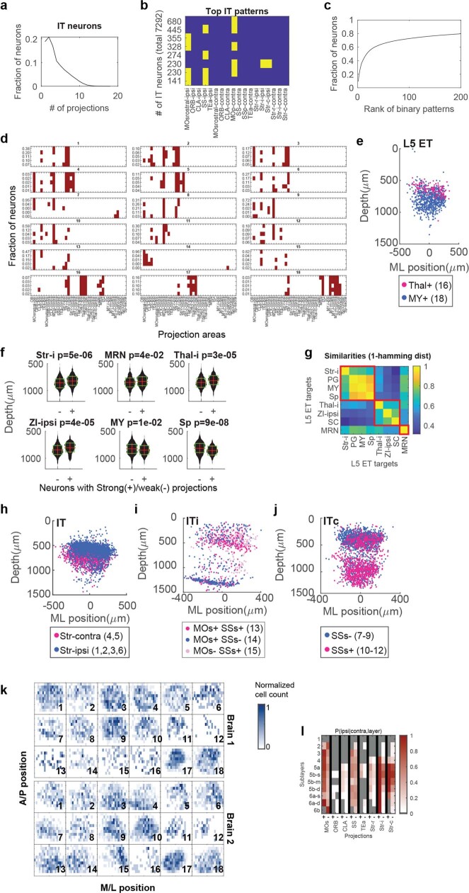
An essential step toward understanding brain function is to establish a structural framework with cellular resolution on which multi-scale datasets spanning molecules, cells, circuits and systems can be integrated and interpreted¹. Here, as part of the collaborative Brain Initiative Cell Census Network (BICCN), we derive a comprehensive cell type-based anatomical description of one exemplar brain structure, the mouse primary motor cortex, upper limb area (MOp-ul). Using genetic and viral labelling, barcoded anatomy resolved by sequencing, single-neuron reconstruction, whole-brain imaging and cloud-based neuroinformatics tools, we delineated the MOp-ul in 3D and refined its sublaminar organization. We defined around two dozen projection neuron types in the MOp-ul and derived an input-output wiring diagram, which will facilitate future analyses of motor control circuitry across molecular, cellular and system levels. This work provides a roadmap towards a comprehensive cellular-resolution description of mammalian brain architecture.

Fig. 1. Delineation of the MOp-ul region and its cell-type organization.

a, Brains with different anatomical labelling modalities (Nissl-stained: n = 3; AAVretro-labelled cervical spinal projecting neurons: n = 2; Cre reporter expression, n = 1 for Vglut1 and Vglut3) were co-registered in the CCF average template and viewed in Neuroglancer to facilitate delineation of MOp-ul borders. b, MOp-ul delineation based on combinatorial Nissl-stained cytoarchitecture (left) (Extended Data Fig. 2) and regional and laminar distributions of AAVretro labelling and Cre expression (middle). A triple-injection strategy was used to further validate distinctive projections of MOp-ul versus adjacent SSp-ul and MOs (right, n = 3 for each injection). AAV-RFP (red), PHAL (pink) and AAV-GFP (green) were injected into the MOs, MOp-ul and SSp, respectively (inset, right), revealing mostly non-overlapping terminal fields in the thalamic nuclei, mediodorsal nucleus (MD), CL, PCN and PO (Extended Data Fig. 5). Scale bars, 500 µm. c, The MOp-ul was rendered in 3D within the CCF. d, Left, schematic showing classification of cortical projection neuron types based on their laminar positions, projection neuron class (IT, PT and CT), and specific projection targets. Right (top), analysis of the MOp-ul layer organization by hierarchical clustering of soma depth for retrogradely labelled cells and Cre driver data (Extended Data Fig. 3). Bottom, clustering dendrogram based on MOp-ul soma depth grouped every 25 µm. ACA, anterior cingulate area; MY, medulla; RN, red nucleus.

Fig. 2. Brain-wide MOp-ul projection patterns by layer and class.

a, Key shows tracer types, mouse lines and layer and projection class selectivity for Cre driver lines used to label axons from MOp neurons. Numbers in brackets represent the number of tracer injection experiments per type. Symbols and colour code are used in b–d. b, Injection sites are plotted on a top-down view of the right cortical hemisphere from CCFv3 with the MOp-ul delineation from Fig. 1 in white. Distance between injection sites is 443.0 ± 185.04 μm (mean ± s.d.). c, A directed, weighted connectivity matrix (15 × 628) from MOp to 314 ipsilateral and 314 contralateral targets for each of the fifteen mouse lines or tracers listed in a. Each row shows the fraction of the total axon measured from a single experiment or the average when n > 1. Rows are ordered by major brain division. For AAV1-Cre monosynaptic tracing, known reciprocally connected regions are coloured grey. We performed hierarchical clustering with Spearman rank correlations and complete linkages, splitting the resulting dendrogram into four clusters. AAV1-Cre was not included in the clustering owing to the many excluded regions. A subset of target regions is indicated. The colour map ranges from 0 to 0.01 and the top of the range is truncated. d, Schematic summarizing all major MOp outputs by area, layer and projection class on a whole-brain flat map (Extended Data Fig. 14). ACB, nucleus accumbens; AUD, auditory area; BAC, bed nucleus of the anterior commissure; CB, cerebellum; cc, corpus callosum; CLA, claustrum; DN, dentate nucleus; ENTl, entorhinal area, lateral part; FN, fastigial nucleus; GP, globus pallidus; GRN, gigantocellular reticular nucleus; GU, gustatory areas; HY, hypothalamus; HPF, hippocampal formation; IO, inferior olivary complex; IP, interposed nucleus; IRN, intermediate reticular nucleus; IZp, spinal cord intermediate zone; MARN, magnocellular reticular nucleus; MDRNd, medullary reticular nucleus, dorsal part; MOp-ll, primary motor area, lower limb; MOp-tr, primary motor area, trunk; OLF, olfactory areas; ORB, orbital area; PL, prelimbic area; POST, postsubiculum; PPN, pedunculopontine nucleus; PRNc, pontine reticular nucleus, caudal part; RE, nucleus of reuniens; RR, midbrain reticular nucleus, retrorubral area; SCm, superior colliculus medial zone; sp, spinal cord; SI, substantia innominata; SNr, substantia nigra, reticular part; SPVO, spinal nucleus of the trigeminal, oral part; SSp-ll, primary somatosensory area, lower limb; SSp-m, primary somatosensory area, mouth; SSp-tr, primary somatosensory area, trunk; STN, subthalamic nucleus; TTd, taenia tecta, dorsal; VTA, ventral tegmental area; ZI, zona incerta. Source data

Fig. 3. Brain-wide inputs to MOp-ul by layer and class.

a, Key shows tracer types, mouse lines and layer and projection class selectivity for Cre driver lines used to label inputs to MOp neurons. Numbers in brackets represent the number of tracer injection experiments per type. Symbols and colour code are used in b–d. b, Injection sites are plotted on a top-down view of the right cortical hemisphere from CCFv3 with the MOp-ul delineation from Fig. 1 in white. Distance between injection sites is 622.4 ± 337.01 μm (mean ± s.d.). c, A directed, weighted connectivity matrix (26 × 628) to MOp from 314 ipsilateral and 314 contralateral targets for each of the mouse lines or tracers listed in a. Each row shows the fraction of the total input signal measured from a single experiment or the average when n > 1. Rows are ordered by major brain division. We performed hierarchical clustering with Spearman rank correlations and complete linkages, splitting the resulting dendrogram into two major clusters (rabies + CTB and TRIO experiments). A subset of input regions is indicated. The colour map ranges from 0 to 0.01 and the top of the range is truncated. d, Schematic summarizing major MOp inputs by area (red), layer (L5 IT Tlx3⁺ neurons, green), and target-defined projection class (CP-projecting neurons, blue) on a whole-brain flat map. The sizes of dots represent relative connectivity strength. AId, agranular insular area, dorsal part; AM, anteromedial nucleus; AUDv, ventral auditory area; bfd, barrel field; CEAl, central amygdalar nucleus, lateral part; CM, central medial nucleus of the thalamus; inh, inhibitory; LHA, lateral hypothalamic area; NDB, diagno band nucleus; proj, projecting; RSP, retrosplenial area; Ssp-bfd, primary somatosensory area, barrel field; VPL, ventral posterolateral nucleus of the thalamus. Source data

Fig. 4. Projection mapping with single-cell resolution using BARseq.

a, log-transformed projection patterns of 10,299 neurons mapped in the motor cortex. Rows indicate single neurons and columns indicate projection areas. See Supplementary Information for a detailed list of dissection areas. Colour bar indicates log of barcode counts. b, Scatter plot of soma locations of the mapped neurons in the cortex. The x-axis indicates relative medial–lateral positions, and the y-axis indicates laminar depth. Neurons are coloured by major classes as indicated. c, Mean projection strengths of the indicated subgroups. Rows indicate projection areas and columns indicate subgroups. Top, dendrogram constructed from the distance of mean projection patterns, with major classes and splits indicated. Bottom, histograms of the laminar distribution of subgroups. Sublayer identities as defined in Fig. 1d are indicated on the right, and sublayer boundaries are indicated by dashed lines. d, The most enriched subgroup (yellow) and the second most enriched subgroup (light blue) in each sublayer. e, Probabilities of projections to the ipsilateral MOs in IT neurons with (top) or without (bottom) contralateral MOs projections in layers L3 to L5b-d. f, The differences in probability for projection X in the indicated sublayer, conditioned on whether the neuron projects to Y. g, Cartoon model showing restricted IT projections in superficial layers and broad IT projections in deep layers. Thal, thalamus. OB, main olfactory bulb. Sp, spinal cord. ITc, intratelencephalic neurons with contralateral projections. ITi, intratelencephalic neurons with only ipsilateral projections.

Fig. 5. Full morphological reconstructions reveal diverse single-cell projection motifs.

a, Soma locations (n = 303) plotted in a top-down view of CCFv3. MOp-ul delineation from Fig. 1 is shown in purple. b, Matrix showing the fraction of total axon projections from tracer (following the colour scheme from Fig. 2a) and single-cell reconstruction experiments to each of 314 targets across all major brain divisions. Columns show individual experiments. Rows show target regions ordered by major brain division. Hierarchical clustering and cutting the dendrogram as indicated with the dashed line revealed thirteen clusters. Some subclusters are indicated by the circled numbers. Cells from specific layers were significantly enriched within clusters (Fisher’s exact test, two-sided, *P < 0.05). c, Top views of all single cells and their axons assigned to cluster 2 (CT), clusters 3 and 4 (ET) and clusters 7 to 13 (IT). Cells are registered to CCFv3, rendered in 3D, overlaid, and randomly coloured (see Extended Data Fig. 20d for single-neuron morphology). d–g, Schematics of single-cell projection targets following visual inspection and classification of motifs. d, Two L6 CT patterns were identified: VAL/PO and VM-dominant projections. e, Four L5 ET motifs are shown: cortico-spinal-, cortico-medulla-, cortico-tectal- and cortico-pontine-dominant patterns. f, g, IT motifs included cells with (+) (g) or without (−) (h) projections to the striatum (STR). f, Bilateral IT motifs include asymmetrical and symmetrical projection patterns. Each schematic shows major projection targets for the cell(s) indicated. cc, corpus callosum; MEA, medial amygdalar nucleus; IMD, intermediodorsal nucleus of the thalamus; MDRNv, medullary reticular nucleus, ventral part; RH, rhomboid nucleus; SPV, spinal nucleus of the trigeminal; SPVI, spinal nucleus of trigeminal nerve, interpolar part. Source data

Fig. 6. Cell type wiring diagram of the MOp-ul.

a, Summary of the output connections of multiple MOp-ul cell types (ET, CT and IT) compared to those of the MOp-ul as a whole (left, black). Along each vertical path, the outputs from one Cre line tracing or single cell reconstruction experiment (identified by the prefix S, followed by a number) are summarized. The outputs begin at top with the originating MOp-ul layer(s); branches perpendicular to the main vertical path that end in ovals represent ipsilateral (right) and contralateral (left) sites of termination, identified by the brain division abbreviations at left. Branch thickness and oval size represent relative connection strength. b, A summary wiring diagram of MOp-ul cell types and predicted functional roles. A subset of cortical and striatal projection patterns is shown from the diverse MOp-ul IT cell types (six IT cell types in L2–L6b). Three types of CT neurons are shown representing different combinations of thalamic targets and MOp-ul layers of origin. Three of four types of ET neurons are also shown, projecting to subcortical targets involved in different motor functions: (1) cortico-spinal outputs to the cervical spinal cord controlling goal-directed upper limb motor activities, such as reaching and grasping; (2) cortico-medullar projections to and output from the reticular formation (for example, medullary reticular nucleus (MDRN)) are implicated in task-specific aspects of skilled motor programs; (3) cortico-tectal projections to the SC are implicated in coordinating movements of eye, head, neck and forelimbs during navigation and goal-oriented behaviours (such as defensive and foraging behaviour) and (4) cortico-pontine projections to the pontine grey, which generates mossy fibres to the cerebellum (which is critically involved in associative motor learning). These ET neurons also generate collateral projections to other structures in the motor system, such as GPe, ZI, STN, RN and IO. ACAv/d, anterior cingulate area, ventral and dorsal part; AIp, agranular insular area, posterior part; AIv, agranular insular area, ventral part; CBN, cerebellar nuclei; CNU, cerebral nuclei; CTX, cortex; MB, midbrain; MDc, mediodorsal nucleus of thalamus, capsular part; NPC, nucleus of the posterior commissure; P, pons; ORBvl/l, orbital area, ventrolateral and lateral part; PARN, parvicellular reticular nucleus; SMT, submedial nucleus of the thalamus; SPFp, subparafascicular nucleus, pavicellular part; TH, thalamus.

Extended Data Fig. 1. Overview of methods, analyses and resources used and generated by the BICCN anatomy group.

Related to Fig. 1. a, Whole brain image data were generated primarily by two automated microscopy methods, STPT and fMOST, and registered in the CCF. Data types include cell type distribution data used for MOp-ul regional delineations (e.g., SERT) and transgenic lines used for projection mapping (e.g., Rbp4-Cre_KL100). Outputs and inputs to MOp-ul were mapped with AAV- and rabies virus-based tracing and BARseq methods. b, Computational approaches used to analyze co-registered datasets include spatial and regional analyses of population labeling to quantitatively describe layer-specific anterograde and retrograde connections, and analyses of single cell morphology reconstructions and BARseq data to derive single neuron projection patterns. Neuroglancer was used for cloud-based data visualization and collaborative analyses of the CCF registered data at high resolution. c, The outcome of these efforts comprise a consensus-based delineation of anatomical borders of the MOp-ul, a detailed description of a cortical layer- and projection neuron type-based wiring diagram, and publicly accessible online data resources. Data and code resources are available at DOI: 10.5281/zenodo.5146390.

Extended Data Fig. 2. Multimodal MOp-ul delineation and validation.

Related to Fig. 1. a, Co-registration of three sets of Nissl staining and other modality data for the delineation of the MOp-ul. (Upper panel) Cloud-based visualization in Neuroglancer of a coronal plane (Bregma +0.5) of three different Nissl brains, ARA, Karten and STPT neurotrace, registered onto CCF at cellular resolution with MOp-ul annotation. (Lower panel) MOp-ul detail of the previous brains overlay to the same markers shown in Fig. 1: Vglut1 and Vglut3 Cre-dependent markers, as well as AAVretro labeled cervical spinal cord projecting neurons. b, Delineations of the MOp based on Nissl-stained cytoarchitecture. The MOp and its adjacent SSp and MOs were delineated based on their areal and laminar cytoarchitectonic properties. The SSp is identifiable with a clearly visible “granular” L4 (gr) consisting of small densely packed somas, which becomes thinner and less granulated (dysgranular or dg) towards its medial tip adjacent to the MOp. Contrary to a general belief that MOp is agranular, we observed a visible thin layer of granular cells that is continued from SSp throughout the MOp. Finally, we identified a transitional junction in L2/3 which was much thinner in MOp than in SSp. Digital images of Nissl-stained histological sections were a gift from Dr. Harvey Karten (http://brainmaps.org/index.php?action=viewslides&datid=43). Manual annotation conducted by Dr. Hong-Wei Dong. c, MOp-SSp boundary algorithmically detection based on Nissl cell textures in 10 brains mapped to the CCF with the borders mapped from CCFv3 (red lines) and CCFv2 (blue lines). c.1, Nissl-based MOp-SSp boundary (at the dorsal surface of the cortex) in 10 brains co-registered to CCF. Each set of bilateral borders with the same color was extracted from one brain. c.2, A sample Nissl stained section around AP +0.8mm. c.3, A magnified view of the region in left hemisphere shown in c.2. c.4, A magnified view of the region in right hemisphere shown in c.2. c.5-c.7, Borders for a section around AP +0.3mm. c.6, In the left hemisphere of the section shown in c.5, an expert-determined MOp-SSp border was denoted in magenta. c.8-c.10. Borders for a section around AP −0.2mm. d, Left: Algorithmically determined boundary (black), and expert manual annotation of the MOp-SSp border (magenta) are shown together with boundaries of reference atlases registered to an individual brain (CCFv2: blue, CCFv3: red). Middle: Results of the algorithmic detection mapped to the CCF. The black lines show the median of the detected MOp-SSp boundaries with 25-75 percentile limits shown in gray. Right: The 25-75 percentile spread as a measure of dispersion (black lines) plotted together with the distances between the reference atlases and the median line (see panel c). e, (Upper panel) Lightsheet microscopic images of 3D whole brain histology. 3D delineation of the MOp layer borders based on whole brain immunostaining with a-NeuN and a-Neurofilament-M (NF-M) using SHIELD-eFLASH. An optical section (left) and zoom-in view (right). (Lower panel) An optical section of the entire brain is shown and 3D rendering of MOp (A, anterior; P, posterior; D, dorsal; V, ventral; M, medial; L, lateral); (Right) The cortical layer borders of MOp delineated based on autofluorescence (black dotted lines) and immunofluorescence (white dotted lines). f, Allen CCF labels, Allen Reference Atlas (ARA) labels, Franklin-Paxinos labels established in the Allen CCF background images. Red signals are from retroAAV-Cre injection in spinal cord registered in the CCF. See details in Supplementary Information for integration of labels from existing atlases onto the Allen CCF. Acronyms defined in Supplementary Table 1.

Extended Data Fig. 3. Connectivity-based MOp parcellation and projection target defined MOp-ul neuron types.

Related to Fig. 1. a, Accuracy of the MOp delineation was further validated using three sets of connectivity data: (1) anterograde axonal projections from the SSp-ul to MOp-ul: transgenic mice (Scnn1a-Tg3-Cre driver line crossed with Ai14 tdTomato reporter line) received an injection of cre-dependent GFP-expressing AAV targeted precisely to the SSp upper limb area (left). Targeting restricted to the SSp was confirmed by the presence of tdTomato fluorescence in SSp layer 4. Analysis using Neuroglancer confirmed the existence of a strong monosynaptic projection from the SSp-ul to MOp-ul, therefore, confirming the border of these two adjacent cortical areas (2nd column of images); (2) the MOp medial border with the MOs was identified by the absence of a monosynaptic MOp connection with the dorsal retrosplenial area (RSPd) and ventrolateral orbital area (ORBvl) and but the presence of strong bidirectional connection between the MOs with both the ORBvl and RSPd3 (the 3rd column of images). b, Detailed distribution patterns of those retrogradely labeled projection neurons in the MOp. Semi-quantitative analysis shows distinct laminar specificities of different neuron types with distinct projection targets. Please also see Extended Data Fig. 7 for additional retrograde labeling in bilateral MOp. Taken altogether, IT neurons are distributed broadly across L2-6 Individual layers contain intermingled IT neurons innervating different targets, and neurons targeting the same structures can be distributed in different layers (also see Fig. 1e; Extended Data Fig. 7). We identified various IT types: 1) two TEa-projecting types: a L2 type that generates an asymmetric projection pattern with denser innervation to the contralateral TEa, and a L5a type with symmetrical projections to bilateral TEa (also see Extended Data Fig. 7); 2) IT neurons that target other ipsilateral somatic sensorimotor areas (e.g. MOs-ul, SSp-ul, MOs and SSs) are intermingled in layers 2, 3, 4, 5a, 5b-middle. These layers also contain dense contralateral MOp-ul PNs and relatively sparse PNs that project to contralateral MOs, SSp and SSs (also see Extended Data Fig. 7a,b); 3) L4 contains many MOs- and SSp-projecting neurons, but far fewer SSs-projecting neurons; 4) L6b IT neurons that project to ipsilateral but not contralateral MOs and SSp (Extended Data Fig. 7b). Cortico-striatal projecting IT neurons are distributed preferentially in L5a and 5b-superficial and -middle (also see Extended Data Figs. 7b). ET neurons are distributed primarily in L5b. Some ET neurons display preferential sublaminar patterns, but other types occur in a smoother gradient across sublayers (also Fig. 1e). Neurons projecting to thalamus (parafascicular nucleus, PF), midbrain (anterior pretectal nucleus, APN; superior colliculus, SC), and hindbrain (pontine nuclei) were preferentially distributed in L5b-superficial and -deep; whereas neurons targeting other regions of the midbrain (red nucleus, RN), the medulla (spinal nucleus of trigeminal nerve interpolar part, SPVI), and cervical spinal cord, were preferentially distributed in L5b-middle and -deep, with the deepest L5b labeling resulting from medulla injections (also see Fig. 1e). Additionally, we identified three classes of L6 CT neurons: (1) L6a neurons that primarily project to the posterior thalamic complex (PO), ventral anterior-lateral thalamic complex (VAL), and PF, as well as the reticular thalamus (RT); (2) VM-projecting neurons in L6a deep sublayer and L6b; and (3) L6b neurons that specifically project to the contralateral thalamic nuclei, such as the PO, VAL and VM (also see Fig. 1e). c, Laminar distributions of retrogradely labeled MOp-ul projection neurons after tracer injections into 13 different projection targets (n=2-4 mice per target). TEa projecting neurons are distributed in L2 and L5a; SSp and MOs projecting neurons are distributed throughout L2-6b; contralateral MOp projecting neurons (commissural neurons) are in L3, L5a and L5b; contralateral CP projecting neurons are in L5a and L5b. All of these neurons belong to the intratelencephalic (IT) neuron type. Several PT (pyramidal-tract neurons) or ET (extratelencephalic) type neurons projecting to the PF, SC, pons, medulla, and spinal cord are in L5b, namely the superficial (L5b-s), middle (L5b-m) and deep (L5b-d). Finally, all corticothalamic projecting neurons (CT) are distributed in superficial L6a (VAL- and PO-projecting neurons), as well as deep L6a and L6b (VM-projecting neurons). d, Representative examples of laminar distribution of cell populations from a subset of cre-driver lines (Cux2, Tlx3, Rbp4, Ntsr1, Ctgf, GAD2, VGat, Pv, Snap25, Vglut1, Vglut3, SERT, Fezf2, Tle4 and PlexinD1, n=6-8 mice per line). See Extended Data Fig. 6 for the complete cre-driver lines laminar distribution.

Extended Data Fig. 4. Distribution of cervical- and lumbar-projecting corticospinal neurons.

Related to Fig. 1. Panels show retrogradely labeled neurons in secondary motor (MOs), primary motor (MOp), and primary somatosensory (SSp) cortical regions following injections of AAVretro-GFP (green) in cervical spinal cord and AAVretro-Cre (red) in lumbar spinal cord in an Ai14-tdTomato Cre-reporter mouse. Values indicate position of coronal sections relative to bregma. Prominent projections to cervical spinal cord arise from anterior MOs (also known as the rostral forelimb area) and more caudally from MOp between +0.7 to +0.1 mm from bregma (also known as the caudal forelimb area). This latter population serves to define the rostro-caudal extent of MOp upper limb domain (MOp-ul), the focus of this study. The lateral aspect of this labeling extends into primary somatosensory area upper limb domain (SSp-ul) and continues caudally to −1.5 mm posterior to bregma. Upper limb-related somatic sensorimotor areas transition into hindlimb- (MOp-ll and SSp-ll) and trunk- (MOp-tr and SSp-tr) related areas caudal to Bregma −0.1 mm, indicated by the increased presence of lumbar-projecting neurons (red). Injection sites in the contralateral cervical and lumbar spinal cord are shown in the bottom right panels. Scale bars, 500 µm.

Extended Data Fig. 5. Distinct output from the MOs, MOp-ul, and SSp-ul.

Related to Figs. 1, 2. Panels show brain-wide axonal projections (a–l) following injections of PHA-L (pink) into MOp-ul, AAV-RFP (red) and AAV-GFP (green) into immediately adjacent MOs and SSp-ul, respectively (injection sites shown in panel c). MOp-ul and SSp-ul project to similar cortical regions (a–e), however they differ in their projections to the thalamus and spinal cord, with SSp-ul uniquely innervating VPL (e, f) and targeting more dorsal layers of spinal cord (l), compared with MOp-ul. In addition, the MOs region just medial to MOp-ul is defined by prominent cortical projections to ORBvl (a, b), RSPd, and PTLp (f), and innervates MD and LP in thalamus (e, f), but lacks a projection to spinal cord (l). Together, these distinct projection profiles demonstrate differences in connectivity that emerge along the medial and lateral borders of MOp-ul. Acronyms are defined in Supplementary Table 1. Scale bars, 1 mm (left panels), 500 µm (right panels, a–l). Please see Supplementary Information for a detailed description of regional output from MOp-ul mapped using PHAL.

Extended Data Fig. 6. Quantitative analysis of Cre expression in newly defined MOp-ul using different cre-driver lines.

Related to Fig. 1. Schematic representation of MOp-ul and cell distribution of Nissl and 33 different cre-driver lines. Quantitative analysis of cortical-depth and layer-based distributions of all different cre-driver lines and Nissl. Cell distributions show specific laminar patterns for all different lines analyzed. Pies represent the percentage of cells in each layer. Interestingly, SERT+ neurons are highly expressed in layer 6 of MOp-ul in contrast to the adjacent SSp area. Similarly, Pdyn+ cells are particularly located in upper layers.

Extended Data Fig. 7. Laminar origin of contralateral MOp projections and distribution of retrogradely labeled TEa, ECT, and/or PERI projecting neurons.

Related to Fig. 1. a, Axonal output to contralateral (left column) and ipsilateral (right column) targets following PHA-L injection in MOp-ul (green). Projections are more prominent in ipsilateral targets, except for TEa, ECT, and PERI regions which receive slightly more input in the contralateral hemisphere (second and third panels from the bottom). b, Laminar distribution and density of cell body labeling in ipsilateral and contralateral MOp following retrograde tracer injections in each of the targets shown in (a). The largest number of cells observed in contralateral MOp arise from injections in striatum (CP), contralateral MOp, and TEa/ECT, mirroring the dense axonal projections to these regions seen in (a). Interestingly, contralateral projections to thalamus appear to arise from cells in the deepest part of L6 (bottom two panels). c, Panels on the left show the laminar distribution of retrogradely labeled cells in ipsilateral and contralateral MOp following retrograde tracer injection in different parts of TEa, ECT, or PERI (right panels). Cell labeling is most prominent in L5a and upper L2/3 and is seen bilaterally or with a contralateral dominance. Scale bars, 500 µm (a, left panels b, c), 1 mm (right panels b, c).

Extended Data Fig. 8. Axon collateral profiles for different target-defined MOp-ul cell populations.

Related to Fig. 1. a, Schematic diagram showing injection strategy. A given downstream target of MOp-ul was injected with either AAVretro-Cre or RVdGL-Cre and MOp-ul was injected with either AAV1-CAG-FLEX-GFP or AAV1-CAG-FLEX-tdTomato to Cre-dependently label the axonal output for each target-defined population. b, Example images of collateral outputs from different MOp-ul projection neuron types. TEa-projecting neurons (first two columns) were found mostly in L5a and collateralized to all cortical targets and striatum, but not to thalamus or brainstem, characteristic of the IT cell class. Interestingly, the striatal projection was predominately ipsilateral, while output to TEa/ECT was bilateral and projections to PERI exhibited a contralateral bias. In contrast, contralateral CP-projecting neurons (third column) also exhibited an IT projection profile, however they were found primarily in L5b (perhaps a result of AAVretro viral tropism), and displayed strong bilateral projections to striatum, but very little projection to TEa, ECT, or PERI regions. Ipsilateral CP-projecting neurons (fourth column) exhibited a similar profile, but also included L5b ET neurons, which project to ipsilateral striatum, as well as thalamus and brainstem regions. Target-defined ET neurons (columns 5-8) broadly collateralized to all other expected targets of this class, except for thalamic-targeting ET cells (column 5, AAVretro-Cre injection in PO labels L5b, but not L6, thalamic projection due to viral tropism) which displayed little or no projection to lateral medulla (e.g. SPVO, last panel in column), while lateral medulla-targeting ET cells (column 8, SPVO) showed little or no projection to thalamus (e.g. PO, fourth panel in column). In addition, all target-defined ET cell populations collateralized to ipsilateral MOs (second row). Lastly, L6 VAL or VM-projecting neurons (columns 9 and 10) co-targeted all other expected thalamic nuclei (PCN, PO, PF) and the reticular thalamic nucleus (RT). No cortical, striatal, or brainstem collaterals were observed, characteristic of the CT cell class. c, Summary of collateral targeting differences for each major cell class. Scale bars, 500 µm (b).

Extended Data Fig. 9. Laminar-specific expression of select genes and transgenic mice.

Related to Fig. 1. Panels show in situ hybridization (ISH) data for endogenous gene expression in MOp taken from the Allen Gene Expression Atlas (http://mouse.brain-map.org/) or for Cre- or Flp-expression in adult transgenic mice (http://connectivity.brain-map.org/transgenic). Data were manually aligned to a representative coronal atlas section through MOp-ul (+0.5mm bregma) and cortical layers are indicated with dashed lines.

Extended Data Fig. 10. Major regions that share reciprocal connections with MOp-ul.

Related to Figs. 1, 2, 3. a, Coronal series of sections highlighting brain regions with both retrograde (CTB, pink) and anterograde (PHA-L, green) labeling following co-injection of both tracers into MOp-ul. Values are in mm relative to bregma. b, c, Higher magnification views (10X) of cortical and thalamic regions shown in (a). This data shows that the MOp-ul shares strong reciprocal connections with (1) other somatic sensorimotor areas (panel b), namely the MOs-ul, contralateal MOp-ul, SSp-ul, SSs and TEa (not shown here); and (2) several thalamic nuclei (c), such as VAL, PO, VM and PF. Scale bars, 1 mm (a), 500 µm (b, c).

Extended Data Fig. 11. Approaches for further establishing synaptic connectivity in downstream targets of MOp.

Related to Fig. 2. a, To distinguish fluorescent labeling of synaptic boutons versus axons of passage in a given MOp target, AAV-hSyn-mRuby2-sypEGFP was injected into MOp-ul and the anterior pretectal nucleus (APN) was examined for the presence of synaptophysin-tagged EGFP+ boutons (green) and mRuby2+ axons (red). b, Injection site in MOp-ul. c, Labeling of boutons and axons in APN at 4X, 10X (d), and 40X magnification (e), confirming synaptic innervation of the downstream structure. f, Similarly, AAV1-hSyn-Cre may be used to confirm and quantify synaptic connectivity in a given target region following anterograde transsynaptic spread of the virus to downstream neurons and subsequent expression of tdTomato in Ai14 Cre-reporter mice. g, Injection site in MOp-ul. h, Post-synaptically labeled tdTomato+ cells (red) in APN at 4X, 10X (i), and 40X magnification (j) confirming a similar pattern of innervation as shown in (d). Blue, fluorescent Nissl stain. Values in mm relative to bregma. Scale bars, 1 mm (b, c, g, h), 200 µm (d, i), 50 µm (e, j).

Extended Data Fig. 12. MOp-ul projection patterns to select targets by layer and class.

Related to Fig. 2. Top row, coronal plane images show the approximate center of each tracer injection site into the MOp-ul area (indicated with *) for wild type mice or Cre lines indicated for each column. Labeled axonal projections are also visible in these sections in the ipsilateral and contralateral CP (CPi, CPc). All other rows, each row shows coronal images at the level of 10 distinct isocortical and subcortical targets of MOp-ul. Anterograde tracing results are strikingly similar across the conventional tracer, PHAL, and AAV-EGFP injected into MOp of wild type mice (first two columns). For some targets (rows) the layer/class origin of the labeled axons in each target is clear. For example, only Cre lines with IT cells project strongly to SSp-ul (Cux2, Rbp4, Tlx3); few to no axons are present in the L5 PT and L6 CT lines. Of note, the hemisphere asymmetry in projections to TEa and PERI is attributable to L2/3 cells, (red boxes in Cux2 column). MOp-ul projections to CEA originate from L5 IT cells (axons labeled in Rbp4 and Tlx3 lines). Ipsilateral VAL projections are strongest in the L6 CT line (Ntsr1), and none of these Cre lines labeled contralateral thalamic projections, although these axons were labeled in both PHAL and wild type AAV tracing experiments. All midbrain projections arise from L5 PT cells (Rbp4, Sim1), as well as the sparse projection to the deep cerebellar nuclei (IP, in Rbp4 panel only). Number of experiments per line and tracer are listed in Fig. 2a (n=1-2; not all experiments were independently repeated as we previously demonstrated n=1 is a good predictor of connectivity strengths across multiple animals). Scale bars = 1 mm in top row panels, 500 μm in all other rows.

Extended Data Fig. 13. Output and input tracing to cell classes in MOp-ul.

Related to Figs. 2, 3. a, b, Maximum intensity projections show the brain-wide distribution of anterogradely labeled axons or retrogradely labeled input cells traced from MOp-ul and from distinct layer and class defined by Cre lines. Note the strong similarities in patterns for all retrograde tracing experiments. c, Frequency distributions of Spearman’s correlation coefficients (R) from the dataset in Fig. 2c and for Rs measured between individual experimental replicates in MOp. A curve was fit to each distribution (lines). The distribution of Spearman Rs between different line-tracer experiments is normally distributed with weaker correlations than for the replicates (mean = 0.30 v 0.79). d, The fraction of total projections is plotted for each line/tracer across 12 major brain divisions. The pie chart inset shows the % of total axons in the PHAL and AAV experiments in WT mice. Most projections from MOp-ul target regions within isocortex, striatum, thalamus and midbrain, with relatively fewer projections to the medulla and pons. The fraction of total projections in each major division reflect the projection class labeled by different Cre lines. For example, L4 IT lines (Scnn1a, Nr5a1) had more axon in isocortex compared to L2/3 and L5 IT lines (1.0 and 0.87 vs. 0.8, 0.74, 0.72, 0.47; Sepw1–L2/3, Cux2–L2/3, Plxnd1–L2/3+L5, and Tlx3-L5, respectively). In contrast, Tlx3–L5 had larger projections into striatum compared to other IT lines (0.53 vs. 0.17, 0.25, and 0.26; Sepw1–L2/3, Cux2–L2/3, and Plxnd1–L2/3+L5, respectively). e, Frequency distributions of Spearman’s correlation coefficients (R) from the dataset in Fig. 3c and for R measured between individual experimental replicates in MOp. A curve was fit to each distribution (lines). Correlations between input patterns for all pairs of lines and tracers (columns in Fig. 3c) were significantly lower than for technical replicates (p=0.02, Kruskal-Wallis test with Dunn’s multiple comparison post hoc). The mean of the distribution of Spearman Rs between retrograde tracing experiments is notably closer to the replicate mean (0.55 v 0.76) compared to the anterograde tracing experiments. f, The fraction of total inputs is plotted for each line/tracer across 12 major brain divisions. The pie chart inset shows the % of total inputs from the CTB experiment in WT mice to summarize the total brain-wide distribution across all layers/classes. Most input to MOp-ul is from regions within isocortex, followed by thalamus across all lines/tracers.

Extended Data Fig. 14. Schematic summaries of MOp-ul outputs by area (PHAL) and for different cell types revealed with cre-dependent AAV tracing in different cre mouse lines on a whole brain flatmap of the rodent brain5 (also see Swanson, Brainmap 4.0 in http://larrywswanson.com/?page_id=1415).

Related to Fig. 2. These data shows that each of the MOp cell types (L2/3 IT, L4 IT, L5 IT, L5 ET/PT, L6 CT) display a discrete subset of MOp projections. Please note that these results also showed MOp-ul axons targeting several previously unreported areas, e.g., the capsular central amygdalar nucleus (CEAc), bed nucleus of the anterior commissure (BAC), globus pallidus external segment (GPe), contralateral thalamic nuclei (PCN), and cerebellar interposed nucleus (IP; Suppl. Information). Further analyses of the connectivity matrix (Source Data Fig. 2, formatted matrix tab) and images (Extended Data Fig. 12) reveal the predominant PN types constituting new and established MOp-ul output channels (also see Fig. 2d). For example, projections to SSp-ul originate from both L2/3 and L5 IT neurons labeled in the Cux2–L2/3, Rbp4–L5 and Tlx3-L5 populations. Projections to CEAc arise from L5 IT cells (Rbp4-L5 and Tlx3-L5, also see Extended Data Fig. 12), and projections to GPe are primarily from ET cells (Rbp4-L5, Fezf2-L5, Foxp2-L6, Sim1-L5). Anterograde experiments also confirmed (in Cux2-L2/3) the population of L2 neurons projecting contralaterally to TEa, ECT, and PERI identified by retrograde tracing (see Extended Data Fig. 7), and a Tle4-L6 CT projection to contralateral thalamic nuclei. Moreover, the sparse cerebellar projection to the IP nucleus we observed with PHAL, AAV-GFP, and AAV1-Cre anterograde monosynaptic tracing is also labeled in Rbp4-L5, but not other ET lines (Source Data Fig. 2, Extended Data Fig. 12).

Extended Data Fig. 15. Brain-wide input patterns from select sources to MOp-ul by layer and class.

Related to Fig. 3. Top row, coronal plane images show the approximate center of each tracer injection site into the MOp-ul area (indicated with *) for wild type mice or Cre lines indicated for each column. The number of starter cells varies by Cre line for the rabies experiments and is shown in the injection panels. All other rows, each row shows coronal images at the level of three distinct source locations with cells that send input to MOp-ul. Number of experiments per line and tracer are listed in Fig. 3a (n=1-2). Scale bars = 1 mm in top row panels, 500 μm in all other rows.

Extended Data Fig. 16. Neural inputs to the MOp.

Related to Fig. 3. a, TRIO experiments reveal monosynaptic input to projection-defined MOp cell types. (Upper panel) Schematic diagram of TRIO approach. AAVretro-Cre is injected into a downstream target of a MOp projection neuron population (ex. CP) and Cre-dependent, TVA- and RG-expressing helper virus (AAV8-hSyn-FLEX-TVA-P2A-GFP-2A-oG) and mCherry-expressing G-deleted rabies virus are injected into the MOp to label the MOp projection neurons population (1^st-order) and their brain-wide monosynaptic inputs (2^nd-order). (Lower panel) Example images of three separate TRIO experiments identifying monosynaptic inputs to IT, PT, and CT cell classes within the MOp showing Cre injection sties (left), helper virus and rabies injection sites in MOp (middle), and monosynaptically labeled inputs in the SSp and thalamus (right). b, Axonal projections to the MOp-ul arising from different cortical areas and thalamic nuclei display diverse laminar specificities in the MOp-ul. For example, MOs axons are preferentially distributed in L1, L5 & L6; densest TEa axons are primarily distributed in L6b; while axons from SSs and contralateral MOp are distributed diffusely across all layers of MOp-ul. Thalamocortical projections to the MOp-ul more or less follow a rough core/matrix organization described previously for thalamic inputs to primary sensory cortices. In particular, VAL axons generate dense terminals specifically in MOp-ul L4, L5b & L6—a typical “core” type thalamocortical inputs. But, axonal inputs from the PO and PF in the MOp-ul are densely distributed in both L1 (a typical “matrix” type inputs) and L4, thus, a mixture core and matrix pattern. PF axons are further distributed in L6. Inputs from other thalamic nuclei, such as VM, MD, and PCN are diffusely distributed across multiple layers. Based on these results, it is reasonable to anticipate that different PN neuron types (IT, PT, and CT) with their soma and dendritic arbor distributions in different layers may preferentially receive discrete cortical and thalamic inputs at single neuron resolution.

Extended Data Fig. 17. related to Fig. 3. Local morphometric features of MOp neurons across layers.

a, Examples of reconstructed cells within MOp cortical layers 2/3/4 (orange) and 5 (blue) (see Methods). Note some L4-5 Cux2/Etv1 neurons lack an apical branch. The total neurons reconstructed for each mouse strain are: MORF3 (@UCLA/USC) x Cux2-CreERT2 (n=9) or Etv1-CreERT2 (n=36); TIGRE-MORF (@AIBS) x Cux2-CreERT2 (n=16), Fezf2-CreERT2 (n=3), or Pvalb-Cre (n=4). b, Principal component analysis (PCA) shows segregation of MOp layer-specific neurons based on measured morphological features. c, Wilcoxon Signed-Rank tests were run (all parameters survived the false discovery rate correction) and group differences between layers 2/3/4 and 5 basal dendritic trees of UCLA/USC (L2-4 [n=11], L5 [n=34]) and AIBS (L2-4 [n=16], L5 [n=7]) cases separately are presented in whisker plots and the degree of their significance is indicated by stars. d, Sholl-like analysis comparing basal dendritic patterns in MOp layer 5 and layers 2/3/4 neurons. The distribution of normalized dendritic length is plotted against the relative path distance from the soma. The graph shows that dendrites of neurons within layer 5 of MOp have slightly larger dendritic length closer to the cell body compared to the dendrites of layers 2/3/4 neurons. e, Persistence-based neuronal feature vectorization was also applied to summarize pairwise differences between superficial and deep neurons for UCLA/USC and AIBS datasets independently. For whisker plots in c and e, the center line represents the median, box limits show the upper and lower quartiles and the whiskers represent the minimum and maximum values.

Extended Data Fig. 18. related to Fig. 4. BARseq projection mapping in MOp compared to other data modalities.

a, Violin plots of the distribution of neurons with the indicated projections across cortical layers. Red crosses and green squares indicate means and median values, respectively. b, Mean normalized projection strengths of neurons in the indicated sublayers. Projection strengths were normalized so that the standard deviation for a projection across all neurons was 0. Black diamonds indicate p < 0.05 for the distribution of the projection strengths in the two adjacent sublayers using two-tailed rank sum test after Holms-Bonferroni correction. p values before correction are shown in Source Data Fig. 2. c, d, Projection patterns from single-cell tracing (c) and BARseq (d) shown at a common resolution achieved by both datasets. e, f, t-SNE plots of combined BARseq and single-cell tracing datasets color-coded by combined cluster classes (e) or by datasets (f). g, Number of neurons in each combined clusters that belong to each dataset. h, i, MetaNeighbor analysis of subgroups of all neurons (h) or IT neurons (i) identified by BARseq and tracing. Higher scores reflect stronger similarity between clusters. j, k, Similarity of sub-sampled BARseq and tracing neurons of the indicated clusters to their cluster centroids (j) or to the centroids of the matching clusters in the other dataset (k).

Extended Data Fig. 19. related to Fig. 4. BARseq projection mapping in MOp.

a, Distribution of projection numbers of IT neurons. b, Top binary projection patterns of IT neurons. The number of neurons with each pattern is indicated on the left. c, Cumulative fractions of IT neurons (y-axis) with the indicated number of binary projection patterns (x-axis). The projection patterns are sorted by their abundances, so the most common patterns are on the left. d, The 5 most abundant binary projection patterns in each subgroup. The fractions of neurons are indicated on the left and the subgroup numbers are indicated on top of each graph. e, Scatter plot of soma locations of the indicated subgroups in the cortex. X-axes indicate relative medial-lateral positions, and y-axes indicate laminar depth. Group numbers are shown in parentheses. Major classes to which the neurons shown belonged to are indicated above each panel. f, laminar distribution of neurons in group 18 with strong (+) or weak (-) projections to the indicated areas. P values using two-tailed rank sum tests after Bonferroni correction are shown on top of each panel. g, similarities between projection targets of L5 ET calculated. The similarity is defined as one minus the hamming distance between two areas based on their binarized co-innervation pattern across neurons of both group 16 and 18. Red squares indicate clusters identified by louvaine community detection. h, i, j, The soma locations of the indicated subgroups of neurons. X-axes indicate relative medial-lateral positions, and y-axes indicate depth. Neurons are colored by subgroups as indicated. Subgroup numbers are shown in parentheses. k, Density maps of each subgroup of neurons on the tangential plane. Neurons from the two brains are shown separately to distinguish labeling bias from real biases in distribution. The density maps are normalized so that the highest density is 1 in each plot. Subgroup numbers are indicated on each plot. l, The projection probability for the indicated ipsilateral projection (x-axis) conditioned on whether the neuron project to the same contralateral area in the indicated sublayer (y-axis).

Extended Data Fig. 20. related to Fig. 5. Single neuron reconstruction data.

a, Digital images (left panel) show two coronal planes (2401 and 2501) through the viral injection site in one representative case (195409). The sections were counterstained with propidium iodide-stained (PI) cellular nuclei to reveal cytoarchitectonic background and facilitate identification of soma locations of labeled neurons. Four L2/3 IT neurons (#03, 06, 23, 24), one L5 ET (#01) and one L6 (#22) neurons were selected for reconstruction. Scale bars, 500 µm. b, c, Analyses of projection target patterns for MOp neurons from the MouseLight dataset and schematic of cell type specific networks. b, Schematic depiction of the major targets contacted by three MOp cells (identified by their MouseLight name) and the pairwise comparisons to quantify the differences in regions targeted (Δ values to the right). c, Histogram of pairwise differences in regions targeted by MOp neurons (“real”) compared to those with randomized targeted regions while normalizing the number of regions invaded by each neuron and the number of neurons invading each region (“shuffled”). The real distribution is broader than the shuffled distribution (CV_shuffled=0.431, half-height-width_shuffled=25; CV_real=0.479, half-height-width_real=31; half-height widths pairs of horizontal arrows) and the statistical difference is highly significant (1-tailed Levene’s test of variances: p < 10⁻²⁵). The left tail reflects similarity between neurons likely in the same projection class; the right to differences between neurons from different classes. d, Top views of the CCF show the brain-wide reconstructions rendered in 3D from example Cre line tracer experiments (colored by layer and projection class key) or individual single cells (red) assigned to each cluster.

Extended Data Fig. 21. MOp-ul regional & cell type networks.

MOp-ul shares extensive bidirectional connections with other cortical areas, including bilateral projections to MOs, SSp, SSs, TEa, and to the contralateral MOp. Although MOp-ul is considered as a single gray matter region node (macroscale), the more than 15 IT projection neuron types revealed here suggest a very complex network at the mesoscale. Two network schematics show three general categories of IT cell type-specific connections: (1) single target types (black arrows, one target, e.g., MOp-ul to MOs); (2) broadcasting types, in which one cell type innervates many cortical targets of MOp-ul (red); (3) multiple combinatorial targets types, in which one cell type projects variably to several targets. Note that in this model and in the case of multiple models coexisting, each cortical target receives inputs from multiple types of MOp-ul IT neurons.

References

1. Swanson LW, Lichtman JW. From Cajal to connectome and beyond. Annu. Rev. Neurosci. 2016;39:197–216. doi: 10.1146/annurev-neuro-071714-033954. - DOI - PubMed
1. Glasser MF, et al. A multi-modal parcellation of human cerebral cortex. Nature. 2016;536:171–178. doi: 10.1038/nature18933. - DOI - PMC - PubMed
1. Zingg B, et al. Neural networks of the mouse neocortex. Cell. 2014;156:1096–1111. doi: 10.1016/j.cell.2014.02.023. - DOI - PMC - PubMed
1. Oh SW, et al. A mesoscale connectome of the mouse brain. Nature. 2014;508:207–214. doi: 10.1038/nature13186. - DOI - PMC - PubMed
1. Hahn, J. D. et al. An open access mouse brain flatmap and upgraded rat and human brain flatmaps based on current reference atlases. J. Compar. Neurol. (2020). - PMC - PubMed
Publication types
Grants and funding
LinkOut - more resources