. 2021 Oct;598(7879):174-181.
doi: 10.1038/s41586-021-03941-1. Epub 2021 Oct 6.

Morphological diversity of single neurons in molecularly defined cell types

Hanchuan Peng #  1   2 Peng Xie #  3 Lijuan Liu #  3   4 Xiuli Kuang  5 Yimin Wang  3   6 Lei Qu  3   7 Hui Gong  8   9 Shengdian Jiang  3 Anan Li  8   9 Zongcai Ruan  3 Liya Ding  3 Zizhen Yao  10 Chao Chen  5 Mengya Chen  6 Tanya L Daigle  10 Rachel Dalley  10 Zhangcan Ding  3 Yanjun Duan  3 Aaron Feiner  10 Ping He  6 Chris Hill  10 Karla E Hirokawa  10   11 Guodong Hong  3   4 Lei Huang  3 Sara Kebede  10 Hsien-Chi Kuo  10 Rachael Larsen  10 Phil Lesnar  10 Longfei Li  7 Qi Li  6 Xiangning Li  8   9 Yaoyao Li  5 Yuanyuan Li  7 An Liu  3   4 Donghuan Lu  12 Stephanie Mok  10 Lydia Ng  10 Thuc Nghi Nguyen  10   11 Qiang Ouyang  3 Jintao Pan  3 Elise Shen  10 Yuanyuan Song  3 Susan M Sunkin  10 Bosiljka Tasic  10 Matthew B Veldman  13 Wayne Wakeman  10 Wan Wan  7 Peng Wang  6 Quanxin Wang  10 Tao Wang  7 Yaping Wang  3 Feng Xiong  3 Wei Xiong  5 Wenjie Xu  10 Min Ye  5 Lulu Yin  3 Yang Yu  10 Jia Yuan  3   4 Jing Yuan  8   9 Zhixi Yun  3 Shaoqun Zeng  8 Shichen Zhang  3 Sujun Zhao  3 Zijun Zhao  3 Zhi Zhou  10 Z Josh Huang  14   15 Luke Esposito  10 Michael J Hawrylycz  10 Staci A Sorensen  10 X William Yang  13 Yefeng Zheng  12 Zhongze Gu  3 Wei Xie  3   4 Christof Koch  10 Qingming Luo  8   16 Julie A Harris  10   11 Yun Wang  10 Hongkui Zeng  17
Affiliations

Morphological diversity of single neurons in molecularly defined cell types

Hanchuan Peng et al. Nature. 2021 Oct.

Abstract

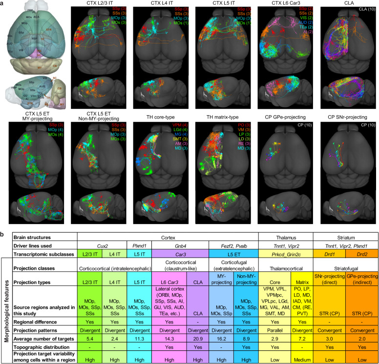
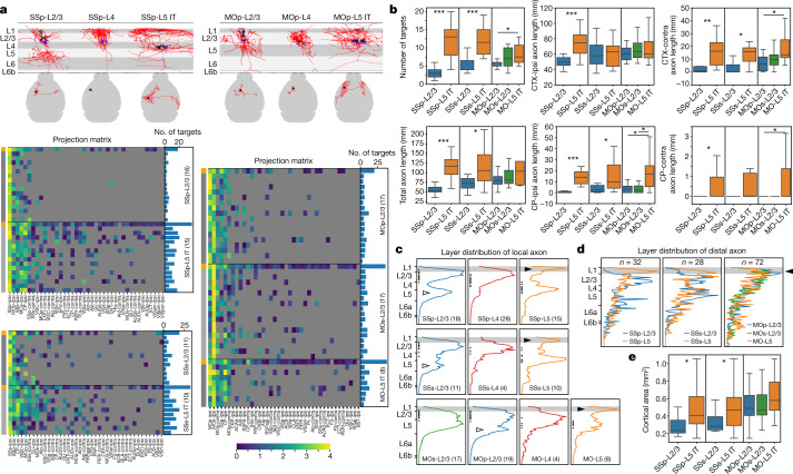
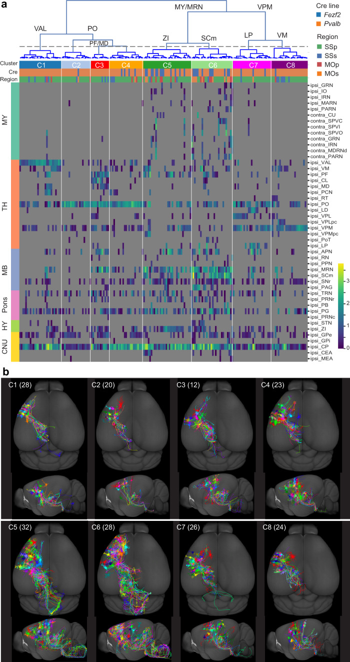
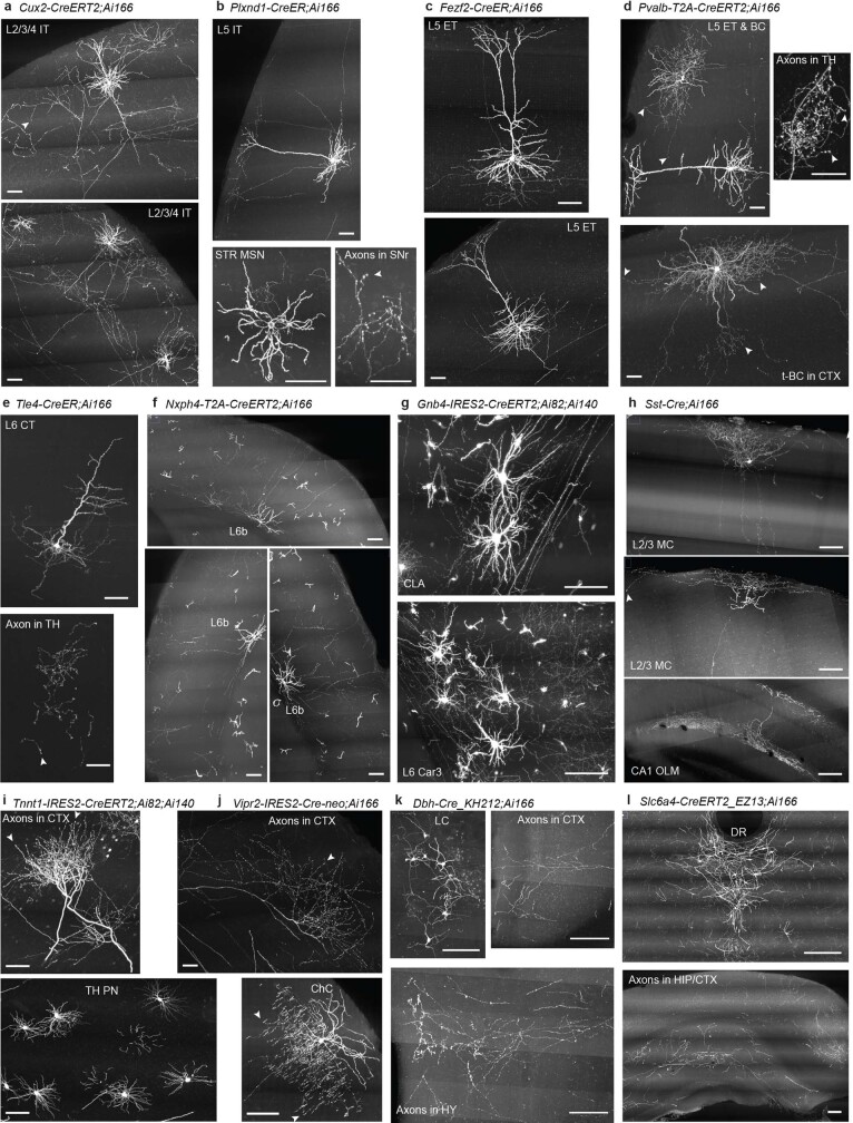
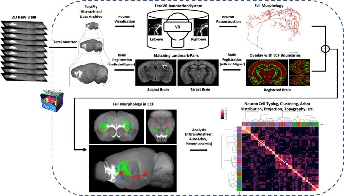
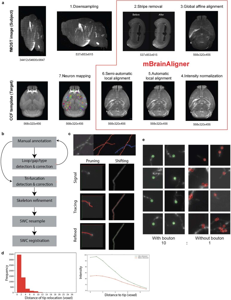
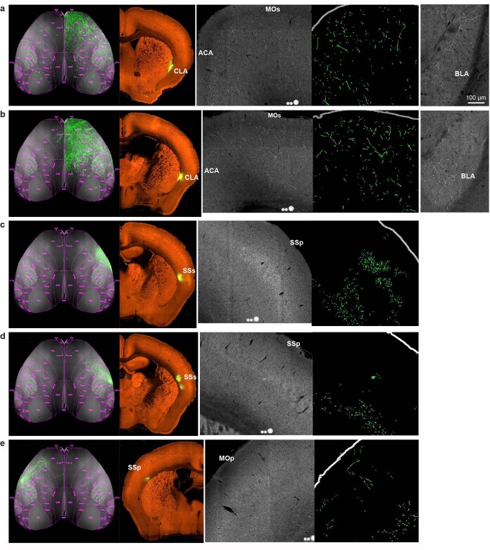
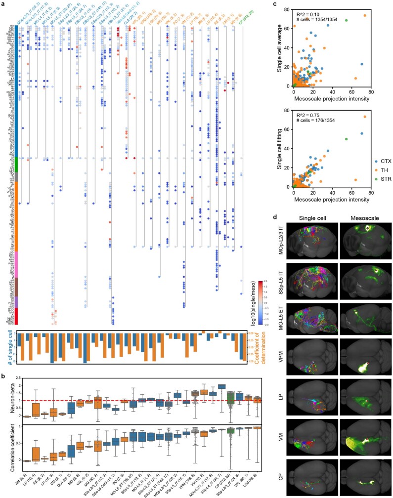
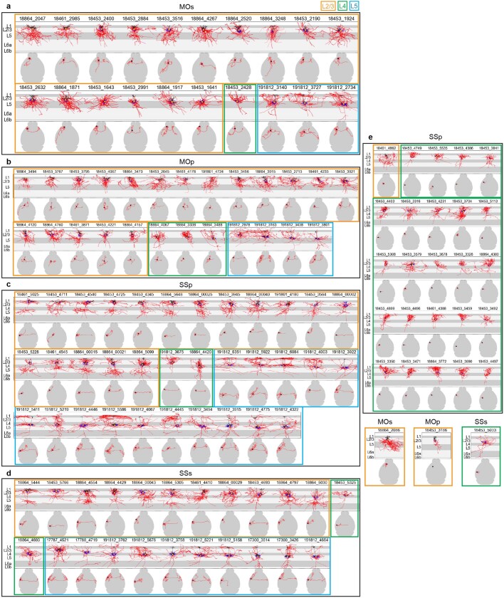
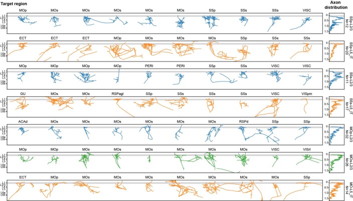
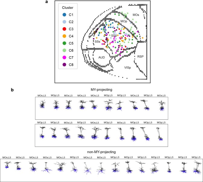
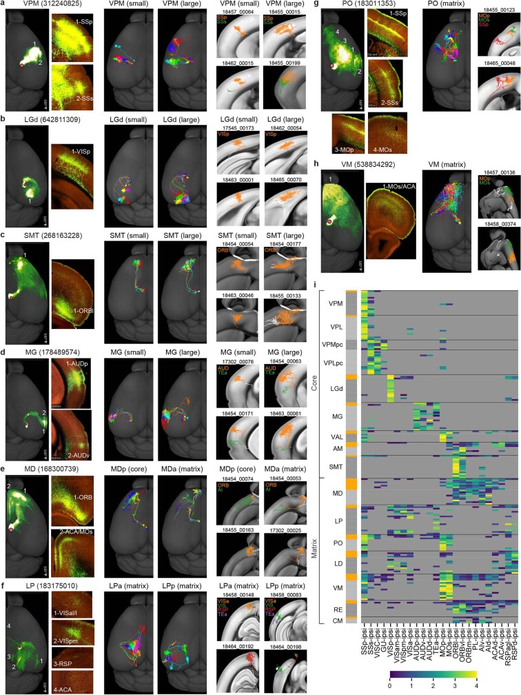
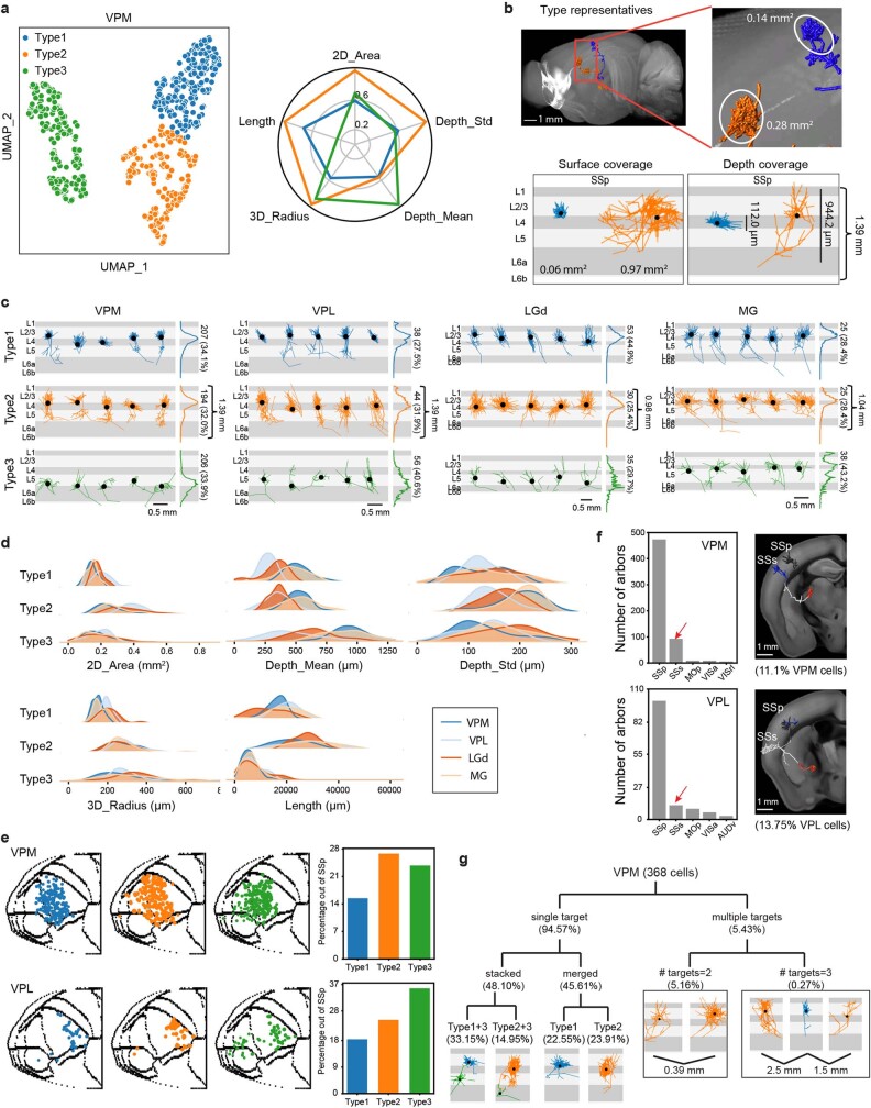
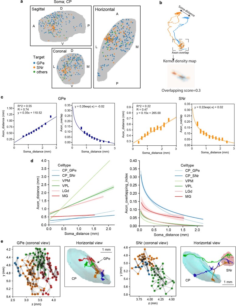
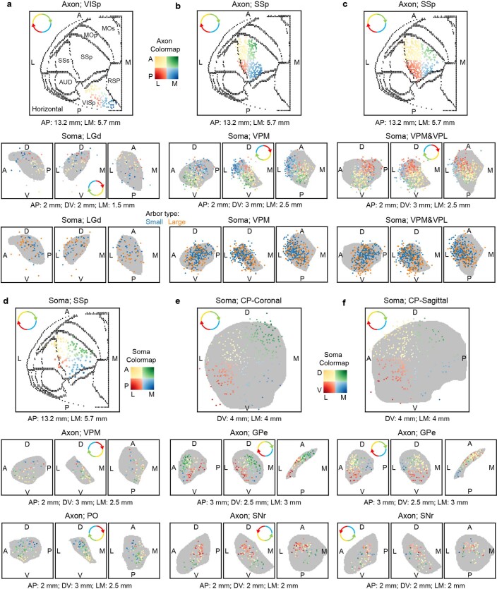
Dendritic and axonal morphology reflects the input and output of neurons and is a defining feature of neuronal types1,2, yet our knowledge of its diversity remains limited. Here, to systematically examine complete single-neuron morphologies on a brain-wide scale, we established a pipeline encompassing sparse labelling, whole-brain imaging, reconstruction, registration and analysis. We fully reconstructed 1,741 neurons from cortex, claustrum, thalamus, striatum and other brain regions in mice. We identified 11 major projection neuron types with distinct morphological features and corresponding transcriptomic identities. Extensive projectional diversity was found within each of these major types, on the basis of which some types were clustered into more refined subtypes. This diversity follows a set of generalizable principles that govern long-range axonal projections at different levels, including molecular correspondence, divergent or convergent projection, axon termination pattern, regional specificity, topography, and individual cell variability. Although clear concordance with transcriptomic profiles is evident at the level of major projection type, fine-grained morphological diversity often does not readily correlate with transcriptomic subtypes derived from unsupervised clustering, highlighting the need for single-cell cross-modality studies. Overall, our study demonstrates the crucial need for quantitative description of complete single-cell anatomy in cell-type classification, as single-cell morphological diversity reveals a plethora of ways in which different cell types and their individual members may contribute to the configuration and function of their respective circuits.


Conflict of interest statement

The authors declare no competing interests.

Figures

Fig. 1
Fig. 1. Morphological and projectional properties of 11 long-range projection neuron types at the single-cell level.
a, Example single-neuron morphologies for each of the 11 projection neuron types. Numbers in parentheses denote the number of neurons shown in each indicated region. In this and all subsequent figures, neurons are flipped to the left hemisphere for comparison of axon projection patterns. Left, CCFv3 3D brain models with anatomical delineation of all cortical and selected subcortical regions (striatum (STR), TH, superior colliculus (SC), PG, MY and cerebellum (CB)). b, Summary of the projection neuron types and their morphological and projectional features. Hyphens denote features not investigated in this study. Our transcriptomic study (H.Z. et al., unpublished results) suggests that most of these thalamocortical projection neurons are in the Prkcd_Grin2c transcriptomic subclass, whereas those from nucleus of reuniens (RE) and paraventricular nucleus (PVT) are not. ACA, anterior singulate area; AI, agranular insular area; AM, anteromedial nucleus; AUD, auditory areas; CM, central medial nucleus; GU, gustatory area; IAD, interanterodorsal nucleus; LD, lateral dorsal nucleus; RSP, retrosplenial area; SMT, submedial nucleus; VIS, visual area; VISC, visceral area; VM, ventral medial nucleus; VPMpc, ventral posteromedial nucleus, parvicellular part.
Fig. 2
Fig. 2. Local morphology and long-range projection of cortical L2/3, L4 and L5 IT neurons.
a, Projection matrices comparing long-range projection patterns between individual neurons and mesoscale population-level projections, and between L2/3 and L5 IT neurons in each cortical region. Example SSp and MOp neurons are shown above the matrices, with their local morphologies (top row; apical dendrite in black, basal dendrite in blue, axon in red and soma as an orange dot) and intracortical long-range projections (bottom row; axon in red and soma as a star). The first row of each matrix (labelled orange in the side bar) shows the mesoscale projection pattern for each cell type and region, collapsed from multiple mesoscale experiments. Each of the subsequent rows shows the projection pattern for a single neuron. Bar graphs to the right show the number of projection target regions for each mesoscale or single cell. MOs and MOp L5 IT neurons are grouped together owing to low numbers in each region. Heat map colours represent projection strengths, defined as ln(NPV × 100 + 1) for mesoscale experiments and ln(axon length) for single cells, where NPV is normalized projection volume. Target regions are defined using thresholds of ln(NPV × 100 + 1) > 0.2 for mesoscale experiments and axon length > 1 mm for single cells. Regions below the thresholds are shown in grey. The same definitions are used for all other figures. b, Comparison of numbers of targets and axon lengths between L2/3 and L5 IT neurons across different regions. In all figures, box edges in box plots show 25th and 75th percentiles, the centre line shows the 50th percentile, and bars show 1.5× the interquartile range (75th percentile – 25th percentile). c, Comparison of vertical profiles of local axon projections among L2/3, L4 and L5 IT neurons. Vertical profiles are combined from all neurons in each type and region (with numbers of cells in parentheses). Soma locations are indicated as dots along the left edge of each plot. Black and white arrowheads point to axon projection differences observed in L1 and L5, respectively. d, Comparison of cumulative vertical profiles of distal axon projections in target cortical regions between L2/3 and L5 IT neurons across different source regions. The black arrowhead points to the axon projection difference observed in L1. e, Comparison of the tangential span of distal axon projections in target cortical regions between L2/3 and L5 IT neurons across different source regions. Cell numbers in parentheses in a are used for quantifications in b, e. *P < 0.05, **P < 0.001, ***P < 0.0001, two-sided Mann-Whitney U test, without adjustment for multiple comparison. ACAd, anterior cingulate area, dorsal part; ACB, nucleus accumbens; AId, agranular insular area, dorsal part; AIp, agranular insular area, posterior part; AUDd, dorsal auditory area; AUDp, primary auditory area; AUDv, ventral auditory area; BLA, basolateral amygdalar nucleus; BST, bed nuclei of the stria terminalis; CEA, central amygdalar nucleus; ENTI, entorhinal area, lateral part; EPd, endopiriform nucleus, dorsal part; FRP, frontal pole; FS, fundus of striatum; ORBl, orbital area, lateral part; PIR, piriform area; PL, prelimbic area; RSPagl, retrosplenial area, lateral agranular part; RSPd, retrosplenial area, dorsal part; VISa, anterior visual area; VISal, anterolateral visual area; VISam, anteromedial visual area; VISl, lateral visual area; VISli, laterointermediate visual area; VISp, primary visual area; VISpm, posteromedial visual area; VISpor, postrhinal area; VISrl, rostrolateral visual area; contra, contralateral; ipsi, ipsilateral.
Fig. 3
Fig. 3. Long-range projection of cortical L5 ET neurons.
a, Clustering based on long-range projection targets of L5 ET neurons from all regions (MOs, MOp, SSp and SSs) combined, and projection matrix heat map organized by clustering result. Main target regions driving each cluster division are shown on the dendrogram. The dashed line indicates the threshold for cluster calls. For the projection matrix, columns represent single cells and rows represent target regions. Heat map colours represent projection strengths, defined as ln(axon length). b, Whole-brain-projection overview (top–down and side views) of individual neurons in each cluster (all cells shown for each cluster, numbers of cells in parentheses). APN, anterior pretectal nucleus; CNU, cerebral nuclei; CU, cuneate nucleus; GRN, gigantocellular reticular nucleus; HY,hypothalamus; IO, inferior olivary complex; IRN, intermediate reticular nucleus; MARN, magnocellular reticular nucleus; MDRNd, medullary reticular nucleus, dorsal part; MEA, medial amygdalar nucleus; PAG, periaqueductal grey; PARN, parvicellular reticular nucleus; PB, parabrachial nucleus; PCN, paracentral nucleus; PoT, posterior triangular thalamic nucleus; PPN,pedunculopontine nucleus; PRNc, pontine reticular nucleus, caudal part; PRNr,pontine reticular nucleus; RN, red nucleus; RT, reticular nucleus; SPVC, spinal nucleus of the trigeminal, caudal part; SPVI, spinal nucleus of the trigeminal, interpolar part; SPVO, spinal nucleus of the trigeminal, oral part; STN, subthalamic nucleus;TRN, tegmental reticular nucleus; VPLpc, ventral posterolateral nucleus, parvicellular part; VPMpc, ventral posteromedial nucleus, parvicellular part.
Fig. 4
Fig. 4. Projection diversity of cortical and claustral Car3 neurons.
a, Clustering of Car3 neurons from all regions based on four feature sets: projection pattern, soma location, axon morphology and dendrite morphology. The dashed line indicates the threshold for cluster calls. Only clusters with a minimum of three cells are shown; thus, three cortical cells are omitted. Each cluster is annotated by the main brain regions where somas (black) and axon terminals (red) reside. Regions are selected to represent more than 50% of cluster members. Bi-ipsi, bilateral or ipsilateral. b, Projection matrix with cells sorted by cluster assignment. Columns represent single cells. Rows represent targets, and the number following each target name indicates the dominant cluster ID for the row. Heat map colours represent projection strengths, defined as ln(axon length). We identified four CTX L6 Car3 cells from ECT and several CLA neurons with axon collaterals projecting into amygdala areas, consistent with previous studies,. c, Total number of cortical targets innervated by each neuron grouped by clusters. Two different thresholds are used to label a region as targeted. With a threshold of at least one terminal bouton, we find an average of 18 targets for CLA and 11 for CTX Car3 neurons. Using a minimum of 1 mm of axon length results in 21 and 14 targets for CLA and CTX Car3 neurons, respectively. Cell numbers are shown in d. Whiskers show outliers below minima or above maxima. d, Whole-brain top-down view of neurons in each cluster (all cells are shown for each cluster, with cell number in parentheses). ACAd, anterior cingulate area, dorsal part; ACAv, anterior cingulate area, ventral part; ENT, entorhinal area; ENTm, entorhinal area, medial part; LA, lateral amygdalar nucleus; MO, motor cortex; ORB, orbital area; ORBvl, orbital area, ventrolateral part; PAR, parasubiculum; POST, postsubiculum; RSPv, retrosplenial area, ventral part; SS, somatosensory cortex; SUB, subiculum.
Extended Data Fig. 1
Extended Data Fig. 1. Genetic strategy for sparse, robust and consistent brain-wide neuronal labeling.
a, Schematic diagram showing the first approach of sparse and robust labeling, involving the combination of CreERT2 transgenic driver line or Cre-expressing AAV (1) with the GFP-expressing TIGRE2.0 reporter line Ai139 or Ai140 (2). Very low dose tamoxifen induction of CreERT2 (Supplementary Table 1) or very low-titer AAV-Cre delivery results in activation of the reporter in a spatially sparse manner. Transgenic reporter expression of GFP is robust and consistent across different cells. An optional addition is to cross in the GFP-expressing TIGRE1.0 reporter line Ai82 (3), so that the tTA2 from Ai139 or Ai140 will activate the expression of GFP from two alleles – Ai139/Ai140 and Ai82, further increasing the level of GFP within Cre+ cells. b, Schematic diagram showing the second approach of sparse and robust labeling, involving the combination of Cre or CreERT2 transgenic driver line or Cre-expressing AAV (1) with the GFP-expressing sparse reporter line TIGRE-MORF (Ai166) (2). In TIGRE-MORF (Ai166), the GFPf transgene is not translated at baseline due to the out-of-frame G22 repeat relative to the open reading frame of GFPf, which lacks its own translation start codon. During DNA replication or repair, rare events of stochastic frameshift of the mononucleotide repeat result in correction of the translation frame (i.e., G22 to G21) and produce expression of the GFPf protein in a small subset of cells. Ai166 exhibits a labeling frequency of 1-5% when crossed to different Cre driver mouse lines. Even with this frequency, we find that combining Ai166 with many Cre driver lines densely expressing the Cre transgene does not produce sufficient sparsity to readily untangle the axonal ramifications, whereas combining it with Cre lines that are already relatively sparse, or with CreERT2 lines with intermediate dosing level of tamoxifen (Supplementary Table 1), results in very sparse labeling. The use of membrane associated GFPf also enables robust labeling of very thin axon fibers. Leaky background expression of GFP reported in other TIGRE2.0 lines is not present in Ai166 mice due to the strict dependency of translational frameshift for the expression of GFPf reporter, making Ai166 an ideal reporter line for sparse and strong labeling of various neuronal types across the brain. Our labeling strategy using stable and universal transgenic reporter mouse lines coupled with a variety of sparse Cre delivery methods has several advantages. First, the TIGRE2.0-based transgenic reporter lines, especially Ai166 which expresses a farnesylated GFP, produce very bright GFP labeling of axon fibers under fMOST imaging, revealing numerous terminal boutons, an essential requirement for obtaining truly complete morphologies. Second, this strategy enables sparse labeling across multiple regions within the same brain, improving efficiency compared to other methods (e.g., in vivo electroporation or stereotaxic virus injection). Third, the labeling is highly consistent from cell to cell, cell type to cell type, region to region, and brain to brain, reducing variability and enhancing reproducibility. Finally, sparse Cre recombination can be achieved through the use of transgenic Cre or CreERT2 driver lines labeling any neuronal type, or low-dose Cre viral vectors delivered through either local or systemic (e.g., retroorbital) injections.
Extended Data Fig. 2
Extended Data Fig. 2. Sparse, robust and consistent labeling and visualization of the dendritic and axonal arborizations of a wide range of neuronal types.
Images shown are 100-µm maximum intensity projection (MIP) images (i.e., projected from 100 consecutive 1-µm image planes). Arrowheads indicate observed terminal boutons at the end of the axon segments. Number of fMOST imaged brains per mouse line and tamoxifen induction conditions are shown in Supplementary Table 1. Scale bars, 100 µm. a, Cortical L2/3/4 IT neurons and their extensive local axon collaterals clearly labeled in a Cux2-CreERT2;Ai166 brain. b, Cortical L5 IT neurons and their local axon collaterals seen in a Plxnd1-CreER;Ai166 brain. Striatal medium spiny neurons (STR MSN) are also sparsely labeled, and their individual axons are clearly seen in substantia nigra, reticular part (SNr). c, Cortical L5 ET neurons and their sparse local axon collaterals seen in a Fezf2-CreER;Ai166 brain. d, Cortical inhibitory basket cells (BC) and translaminar basket cells (t-BC), as well as L5 ET excitatory neurons, seen in a Pvalb-T2A-CreERT2;Ai166 brain. The L5 ET neurons form driving-type axon clusters with large boutons in the thalamus (TH). e, Cortical L6 CT neurons and their characteristic apical dendrites not reaching L1, as well as local axon collaterals and long-range axon projections into thalamus (TH), labeled in a Tle4-CreER;Ai166 brain. f, Cortical L6b neurons and their local axon projections up into L1 seen in a Nxph4-T2A-CreERT2;Ai166 brain. g, Gnb4+ claustral (CLA) and cortical (L6 Car3) neurons with their widely dispersed axon fibers seen in a Gnb4-IRES2-CreERT2;Ai140;Ai82 brain. h, Cortical inhibitory Martinotti cells (MC) and hippocampal CA1 OLM cells labeled in a Sst-Cre;Ai166 brain. i, Thalamic projection neurons (TH PN) with their dense axon terminal clusters in cortex seen in a Tnnt1-IRES2-CreERT2;Ai82;Ai140 brain. j, In a Vipr2-IRES2-Cre-neo;Ai166 brain, axon clusters from projection neurons in visual thalamic nuclei are seen in cortex (CTX), and a cortical chandelier cell (ChC) is fully labeled with its characteristic axonal branches. Vipr2-IRES2-Cre-neo;Ai166 also labels axons consistent with projections from retinal ganglion cells, which are not shown here. k, Noradrenergic neurons labeled in the locus ceruleus (LC), and their long-range axon fibers seen in CTX and hypothalamus (HY) in a Dbh-Cre_KH212;Ai166 brain. l, Serotonergic neurons labeled in the dorsal raphe (DR), and their long-range axon fibers seen in hippocampus (HIP) and CTX in a Slc6a4-CreERT2_EZ13;Ai166 brain. Overall, it is apparent that these neurons display a remarkable array of dendritic and axonal morphologies. Specifically, in these sparsely labeled brains, cortical IT, ET and CT neurons not only have primary long-range projections but also local axonal branches that are well segregated and clearly identifiable, enabling truly complete reconstruction of the entire local and long-range, cortical and subcortical axonal arborization (ae). L5 ET neurons form the ‘driving’ type of synapses in the thalamus,, which have enlarged and intensely fluorescent boutons (d). L6b subplate neurons extend their local axon collaterals upwards into layer 1 (f). The axons of thalamic projection neurons form either dense or dispersed clusters in the cortex (i, j). On the other hand, claustral, noradrenergic and serotonergic neurons have widely dispersed, thin axons that are nonetheless well labeled (k, l). One can also clearly see individual axons in the substantia nigra from striatal medium spiny neurons (b), as well as dense and fine local axonal branches of a variety of cortical interneurons (e.g., basket cells, Martinotti cells and chandelier cells) (d, h, j). Of note, sparsely labeled neurons were frequently observed in other regions of the brain for all of these crosses but are not described in detail here. Each of these brains contains ~100-1,000 labeled neurons (Supplementary Table 1). Thus, tens of thousands of neurons could be reconstructed from these and newly generated datasets in the coming years. The whole brain image datasets are publicly available as a unique resource for the community.
Extended Data Fig. 3
Extended Data Fig. 3. Platform and workflow of the brain-wide complete morphology imaging, reconstruction, registration and analysis pipeline.
Each fMOST dataset is first converted to a multi-level navigable TeraFly dataset using TeraConverter, the data formatting tool in the Vaa3D-TeraFly program, which allows smooth handling of terabyte-scale datasets. Neuron visualization and reconstruction is then carried out on the TeraFly files. A series of tools, especially those based on the “Virtual Finger” method, were developed within Vaa3D to facilitate semi-automated and manual reconstruction. Further, a virtual reality (VR) environment created within Vaa3D, TeraVR, significantly enhances a user’s ability to see the 3D relationships among intertwined axonal segments, improving precision and efficiency of reconstruction. Annotators work in the TeraVR annotation system to reconstruct the full morphology of each neuron. After quality control (QC) and manual correction, Vaa3D’s deformable model is used to automatically fit the tracing to the center of fluorescent signals. The final reconstructed morphology is completed as a single tree without breaks, loops, or trifurcations. All these data processing, reconstruction, and workflow control processes are managed using a specific software system for massive scale data production. In parallel, each fMOST dataset is registered to CCFv3 using mBrainAligner, which uses both CLM (Coherent-Landmark-Matching) and LQW (Little-Quick-Warp) modules in brain alignment. Following registration of the whole-brain image dataset to CCFv3, all the reconstructed morphologies from the same brain are also registered for subsequent visualization and quantitative analysis. Registration to CCFv3 enables digital anatomical delineation and spatial quantification of each reconstructed morphology and its compartments (e.g., soma, dendrites, axon arbors). Since neurons are reconstructed from different brains, co-registration to the CCFv3 allows them to be compared and analyzed using a unified framework, mBrainAnalyzer, which automatically detects the arbors of each neuron followed by mapping of these dendritic and axonal arbors onto the standardized CCFv3 space. Morphological features such as length, depth, area, etc., at the whole neuron level are also computed for each arbor-domain for analysis.
Extended Data Fig. 4
Extended Data Fig. 4. CCF registration and QC of reconstructed morphologies.
a, CCF registration workflow. Pipeline of 3D registration from fMOST image (subject) to average mouse brain template of CCFv3 (target). Numbers below each panel indicate the pixel sizes in the order of X*Y*Z. See Methods for explanation of each step. b, Workflow of post-processing process for QC of reconstruction SWC files: 1. automatic detection and correction of basic reconstruction errors including loops, gaps and incorrect node types. 2. Corrections are sent back for manual verification. 3. Automatic detection and correction of trifurcations, which are usually overlapping neurites, instead of branching points. 4. Refinement of SWC files, including pruning of over-traced terminals and shifting skeleton to fit the center of image signals. 5. Resampling of SWC to achieve evenly distributed nodes. 6. SWC registration to the standard CCFv3 mouse brain template. c, Examples of trifurcation before (middle) and after (right) correction (blue and red branches do not cross), and examples of refinement before and after pruning (lower left panels) and shifting (lower right panels). d, Refinement leads to more precisely defined axon termination. Upper, distribution of terminal relocation distance by pruning. Lower, radius-decay curve of terminal signals shows that after refinement the axon ends at a brighter spot (indicating a bouton) rather than tapering off. e, Examples of axon terminals that end with or without a bouton. We established a stringent QC process that includes ensuring the completeness of reconstructed morphologies. A conventional way to assess the completeness of axon labeling and reconstruction is whether an axon ends at a bouton, as indicated by an enlargement with more intense signal (see arrowheads in Extended Data Fig. 2), or gradually tapers off, the former suggesting a complete labeling. We implemented this assessment in our reconstruction refinement process to identify potential inaccuracies. In our final QC-passed reconstructions we found that the ratio between terminal axon branches with and without a terminal bouton was about 10:1, indicating a high degree of completeness of our reconstructed morphologies.
Extended Data Fig. 5
Extended Data Fig. 5. Anterograde bulk AAV tracing of projections from Gnb4+ neurons in claustrum or lateral cortex.
ae, AAV2/1-pCAG-FLEX-GFP tracer was injected into the claustrum (a, b), SSs (c, d) or SSp (e) in Gnb4-IRES2-Cre or Gnb4-IRES2-CreERT2 mice. Brains were imaged by the TissueCyte STPT system. First panel in each row: top-down view of segmented GFP-labeled axon projections in the cortex. Second panel: injection site. Third panel: the fine axon fibers in a target cortical area. Fourth panel: the segmented image of the third panel to visualize and quantify the axon fibers. Fifth panel in a and b: axon fibers observed in basolateral amygdalar nucleus (BLA). Full STPT image datasets are available at the Allen Mouse Brain Connectivity Atlas web portal (http://connectivity.brain-map.org/) with the following experiment IDs: a, 514505957; b, 485902743; c, 553446684; d, 581327676; e, 656688345. These 5 selected datasets were replicates of each other and all had small, spatially specific, injection sites that were located very close to each other. These small bulk injections demonstrate very distinct projection patterns between claustral and cortical Gnb4+ neurons.
Extended Data Fig. 6
Extended Data Fig. 6. Combination of single neuron morphologies recapitulates population-level mesoscale projection patterns.
a, Comparative projection map of single cells and mesoscale experiments. Individual samples are grouped by brain areas and/or cortical layers based on soma locations (single cell) and injection sites (mesoscale). This dataset covers 14 cortical areas and layers combined, 13 thalamic nuclei and one striatal structure (CP). Each group is represented by a stretch of connected dots with ipsilateral and contralateral targets in the two hemispheres, respectively. Projection intensities in each target region are quantified as ln(NPV × 100 + 1) for mesoscale experiments, where NPV denotes normalized projection volume (Supplementary Table 3), and axon lengths within the target region for single cells. Target regions are defined using thresholds of ln(NPV × 100 + 1) > 0.2 for mesoscale experiments and axon length > 1 mm for single cells. Only target regions present in at least 50% mesoscale experiments or 10% single cells are shown here. Dot colors are scaled by the log10 of single-cell and mesoscale strength ratio. Lower panel, coefficients of determination (orange bars) and number of cells (blue bars) of mesoscale regression by single cells (described in c). b, Box plots of neuron-beta and correlation coefficients between single cells and group-average of mesoscale data. Individual comparisons shown as swarm plots overlapped with boxes. Box plot specifications: box bounds = 25th and 75th percentile, center = 50th percentile, minima/maxima = center ± 1.5 × IQR (75th percentile – 25th percentile), no whiskers shown. The first and second numbers in the group labels in a and b indicate the numbers of single cells and mesoscale experiments, respectively. To quantitatively compare the single cell and mesoscale tracer experiments, we calculated the correlation coefficient of each single cell’s brain-wide projection weights with the average projection weights from the location-matched mesoscale experiments. The correlation coefficients range from −0.04 (i.e., AM) to 1.00 (i.e., LGd), with a median of 0.69. High correlation coefficients may indicate simple compositions of projecting patterns, e.g., LGd with almost pure VISp projections and CP projecting mainly to either GPe or SNr. Low correlation coefficients may indicate complex composition of projecting patterns, e.g., AM, RE and CM for reasons mentioned below. To compare single cell projection strength relative to mesoscale data, we developed a ‘Neuron-beta’ metric, as the covariance of a single cell and the average of mesoscale samples, relative to the mesoscale variance. Single cells with Neuron-beta values > 1.5 correlate well with mesoscale data but fluctuate more variably. For example, individual VM neurons are highly diverse but positively correlated with mesoscale data. Small (< 0.5) positive Neuron-beta values result from low correlation of single cell and mesoscale data. For cell types with Neuron-beta values around 1, single cell and mesoscale data appear to be comparable. c, Approximation of mesoscale projections by single cell projection strengths (1,354 cells used) by group-average (upper) or by linear regression (lower). To study how well the mesoscale projection pattern could be broken down to our set of single cells, we performed linear regression with Lasso regularization to reduce the number of single cells with non-zero weights (representative cells). This approach selects a minimal set of single cells and uses weighted summation of single cell axon length to approximate the cell type specific mesoscale axonal weights. The overall coefficient of determination (R2) is 0.75, indicating that mesoscale connectivity is recapitulated well except for the above-mentioned thalamic nuclei. Only 176 out of 1,354 single cells contribute to the regression. These cells represent a minimal set of stereotypes to make up the population level connectivity (see d). Averaging across all single cells shows a low level of approximation (R= 0.10), suggesting highly diverse morphologies and projection patterns among the single cells. d, Visualization of projection patterns constituted by representative cells and mesoscale projection intensities. Overall, the combined single cell projection pattern from a given region (and cortical layer) is highly concordant with that of the mesoscale experiments. There are a few exceptions to this general trend. The combined patterns from single cortical and CLA Car3 neurons collectively project to more targets than mesoscale experiments, likely due to the richer sampling of single neurons across multiple cortical areas and along the entire extent of CLA than the few mesoscale experiments covered. On the other hand, for several thalamic nuclei (e.g., VAL, VM, AM, RE and CM), single neurons collectively have not captured the full projection patterns from mesoscale experiments. This difference could be due to several reasons: (1) since some of these nuclei are small, the mesoscale experiments may include projections labeled from neighboring nuclei so the single cell data may more accurately represent the true output pattern; (2) the number of reconstructed single neurons is still small and may not fully represent all projection types in a given nucleus; (3) the reconstructed neurons may represent only a subset of the cell types located in these nuclei, and there may be other types of projection neurons not labeled in the Cre lines used here.
Extended Data Fig. 7
Extended Data Fig. 7. Local morphologies and long-range intracortical projections of cortical L2/3, L4 and L5 IT neurons.
ad, Comparison of local morphologies (upper panels; apical dendrite in black, basal dendrite in blue, axon in red, soma as an orange dot) and intracortical projections (lower panels; axon in red, soma as a star) for MOs (a), MOp (b), SSp (c) and SSs (d) neurons. L2/3, L4 and L5 IT neurons are marked by orange, green and blue boxes, respectively. The L4-like neurons from MOp and MOs are located between L2/3 and L5 since L4 is not delineated in MOp or MOs in CCFv3. Neurons are ordered based on the depths from pial surface of their somas. Gray shadings mark generic layers; however, it should be noted that due to variation in layer thickness in different parts of the cortical areas, the generic layer marking does not necessarily correlate with each neuron’s precise soma location. The layer assignment of each neuron’s soma location was confirmed by visual inspection of each case. e, Reconstructed neurons without long-range axon projections outside of their soma areas. Vast majority of these neurons are SSp L4 IT. Overall, recent studies by scRNA-seq, MERFISH and Patch-seq showed that transcriptomically defined cortical IT neuron types are organized by layer, but also exhibit a continuous spatial transition along the cortical depth. Here we arrange the L2/3, L4 and L5 IT neurons according to the depth of their soma from the pial surface, and find that within each region, across depths individual neurons exhibit highly variable long-range projection patterns. We identified 26 cells from SSp and 3 cells from SSs to be in L4. L4 cells have either no apical dendrites (i.e., spiny stellate cells) or a simple apical dendrite that does not branch in L1 (i.e., untufted or star pyramid cells), in contrast to the pyramidal L2/3 cells which have tufted or wide-branching apical dendrites in L1. L2/3 cells have local axons branching in L2/3 and downward into L5, whereas L4 cells have local axons mainly projecting up to L2/3. We also found 4 cells from MOp and MOs with these L4-like features – minimal apical dendrites and upward-projecting local axons, suggesting that these are the L4-like cells located in motor cortex that can also be identified transcriptomically. Consistent with prior notion, all but two SSp L4 cells have only local axons but no long-range projections. However, nearly all L4 cells in SSs, MOp and MOs do have axon projections outside of their local area, as we reported before.
Extended Data Fig. 8
Extended Data Fig. 8. Comparison of terminal axon arbor patterns in target cortical regions between L2/3 and L5 IT neurons.
Axon terminals in specific target regions (labeled on top) of L2/3 or L5 IT neurons from SSp (first two rows), SSs (next two rows), MOp and MOs (last three rows). Because not all neurons project to all target regions, axon terminals from any neurons for each target region are combined. For each neuron type from each region, 10 representative axon terminals are shown here, whereas the overall vertical profile of axon distributions (the rightmost panel) is quantified from all axonal terminals (N indicated below each neuron type label). These axon distribution vertical profiles are also presented in Fig. 2d. Due to variation in layer thickness in different parts of the cortical areas, only generic L1 is shaded.
Extended Data Fig. 9
Extended Data Fig. 9. Retro-seq characterization of cortical IT neurons across all layers from MOs, MOp, SSp and SSs.
Transcriptomes of retrogradely labeled neurons were obtained by single cell or nucleus RNA-sequencing and then mapped to our transcriptomic taxonomy to identify the transcriptomic type (shown as clusters at the top and bottom of the dot plot) of each neuron. Cells are grouped by their source region. Within each source region, cells labeled from different projection targets (Injection Target region of interest, ROI) are compared, and found to be assigned to a similar subset of transcriptomic types without major distinction between ROIs. cMOs or cMOp denotes contralateral MOs or MOp, respectively.
Extended Data Fig. 10
Extended Data Fig. 10. Local morphology and long-range projection analysis of cortical L5 ET neurons.
a, Cortical flatmap showing the distribution of cells belonging to each cluster. b, Dendritic morphologies of motor cortex (MOp and MOs) L5 ET neurons separated into medulla (MY)-projecting and non-MY-projecting groups. Apical dendrite in black, basal dendrite in blue. Comparing the dendritic morphologies of MOp and MOs neurons with or without MY projection shows that MY-projecting neurons tend to have denser basal dendrites as well as more extensive and complex apical dendrites that have their first bifurcation points closer to the somas.
Extended Data Fig. 11
Extended Data Fig. 11. Single-cell RNA-seq characterization of Car3 subclass of cortical and claustral neurons.
a, Transcriptomic taxonomy of the entire mouse isocortex and hippocampal formation reveals a distinct branch of Car3 subclass (dashed box). Bar graph shows the distribution of Retro-seq cells within the Car3 subclass b, Enlarged view of the taxonomy part within the dashed box in a shows the distribution of Retro-seq cells in the 3 clusters of the Car3 subclass. c, Neurons from claustrum (CLA) are also entirely mapped to the Car3 subclass. We combined all CLA and cortical Car3 neuron SMART-Seq transcriptomes and re-clustered them to see if more refined cluster segregation could be obtained, resulting in 8 clusters. Dot plot shows the number of cells from each cortical region or CLA contributing to each cluster. d, Remapping of Retro-seq cells from CLA and several cortical regions (TEa-PERI-ECT and SSs) to the 8 new transcriptomic clusters. e, f, Marker gene expression for different clusters is similar between (e) cells contributing to the clustering shown in c and (f) Retro-seq cells shown in d.
Extended Data Fig. 12
Extended Data Fig. 12. Long-range projection patterns of individual thalamic neurons in comparison with mesoscale population-level projections.
ah, Axonal morphologies and projections of reconstructed single neurons compared with population projection patterns for thalamic nuclei VPM (a), LGd (b), SMT (c), MG (d), MD (e), LP (f), PO (g) and VM (h). For each nucleus: left panels, representative mesoscale experiments shown in a maximum projection whole-brain top-down view and individual higher-power images showing axon termination patterns in major target regions; middle panels, representative single neurons shown together in a whole-brain top-down view; right panels, each representative neuron is shown in a chosen plane to best capture the perpendicular (to pial surface) orientation of the main axon arbor with superimposed maximum projection view of the neuron’s axon arbors. The chosen plane can be coronal (for a, b, d), horizontal (for c, e), sagittal (for h) or tilted (for f, g), based on the main cortical target region. Different cortical target regions are indicated by different colors. Small, small axon arbors. Large, large axon arbors. MDa and MDp, or LPa and LPp are the anterior and posterior parts of MD or LP respectively. i, Projection matrix showing comparison of thalamocortical projection patterns between mesoscale experiments and single neurons as well as among individual neurons, for each listed thalamic nucleus. Each row is a mesoscale experiment (labeled in orange in the left side bar) or a single cell (labeled in grey in the left side bar). Heatmap colors represent projection strengths, defined as ln(NPV × 100 + 1) for mesoscale experiments and ln(axon length) for single cells. Target regions are defined using thresholds of ln(NPV × 100 + 1) > 0.2 for mesoscale experiments and axon length > 1 mm for single cells. Regions below the thresholds are shown in grey. Overall, core-type thalamocortical neurons usually have one major axon arbor targeting L4 of the primary sensory or motor cortex of the corresponding modality, i.e., VPM and VPL projecting to SSp, VPMpc to gustatory areas (GU), VPLpc to visceral area (VISC), LGd to primary visual area (VISp), MG to auditory areas (AUD), and VAL to MOp. Reconstructed neurons from AM, SMT and posterior MD also send a single major axon arbor to various parts of orbital cortex (ORB), with a similar mid-layer termination pattern, suggesting these neurons also belong to the “core” projection type. A small fraction of the core-type neurons (5.43% for VPM, 4.05% for VPL, 15.6% for MG, but 0% for LGd) have more than one axon arbor targeting different cortical areas. In the case of these cells in VPM and VPL, usually they have a larger main arbor targeting SSp, and a smaller secondary arbor targeting SSs (a). MG neurons with two or more cortical targets are mostly of the large-arbor type (d). These multi-target MG neurons are more like the matrix-type neurons, showing stronger projections to L1 and L5, located in the associational parts of MG (e.g., MGm) medial to the core relay auditory nucleus, MGd and MGv. Single neurons are assigned to either small-arbor or large-arbor type (Extended Data Fig. 13). Large-arbor neurons account for 32.0% of the total reconstructions from VPM, 31.9% from VPL, 38.9% from LGd and 36.0% from MG. Neurons in SMT are also separable into small- and large-arbor types, whereas the current set of AM neurons all have small arbors and the posterior MD neurons all have large arbors. Matrix-type thalamocortical neurons exhibit a diverse range of projection and morphological patterns. For example, LP neurons preferentially project to two or more higher visual cortical areas. They do not directly project into VISp, 6 out of 16 reconstructed LP neurons has short axon fibers in VISp (average ~2 mm in VISp, substantially below the average of LGd neurons, ~26 mm). LP neurons can be roughly divided into an anterior and a posterior group, consistent with previous functional studies. Posterior LP neurons mainly project to lateral and posterior higher visual areas, whereas anterior LP neurons mainly project to medial and anterior higher visual areas with some extending an axon projection into anterior cingulate cortex (ACA) (f). PO neurons project to both SSp and MOp/MOs. Their axon arbors in these target regions terminate broadly across layers with an apparent preference in L4 and lower L2/3, with 4 out of 7 sending rich axon arbors (> 1 mm) to L1 (g). Neurons in anterior MD appear very different from those in posterior MD and are more similar to those in neighboring nuclei such as IAD and CM. They have multiple axon arbors that target multiple medial and lateral prefrontal cortical areas including prelimbic cortex (PL), ORB and agranular insular cortex (AI) (e). VM neurons have multiple axon arbors, heavily targeting MOp and/or MOs with additional branches targeting various somatosensory areas (h).
Extended Data Fig. 13
Extended Data Fig. 13. Thalamocortical axon arbor analysis.
Clustering of 944 cortical axon arbors from 586 neurons from VPM, VPL, LGd and MG reveal three types of arbors. Two major types of axon arbors target cortical layer 4 (spanning L4 and lower L2/3); a smaller 'type 1' arbor and a larger 'type 2' arbor (cortical area > 0.3 mm2). The 'type 3' arbor terminate in cortical L6; this type is most often a minor collateral originating from the type 1 or type 2 arbor, so we did not use it to classify neurons. a, Clustering result indicates three types of cortical axon arbors in VPM neurons. Left, UMAP representation of VPM axon arbors. Right, polar plot of main features, values as normalized cluster averages. b, Representative (upper) and extreme (lower) examples of VPM cortical arbors. c, Examples grouped by thalamic nuclei and arbor types. In each sub-panel, vertical views are shown for 5 representative arbors, with branch length distribution for all neurons of the same cluster on the right side. Arbor number and percentage of the group are shown on the right side. d, Distribution of features grouped by thalamic nuclei and arbor types. e, Arbor locations of VPM and VPL neurons in 2D cortical map grouped by arbor types. Each dot represents the center of an arbor. Somas with small and large arbors are spatially intermingled in each nucleus. Right panels show percentage of arbors outside of the primary target of VPM or VPL neurons. f, (Left) Counts of VPM or VPL arbors in cortical regions. (Right) Examples of neurons with double arbors, one in SSp and the other in SSs. g, Variation of VPM neurons by arbor composition. ‘Single target’ neurons are described as ‘stacked’ or ‘merged’ by bi-layer or single-layer distribution. The stacked and merged groups can be further separated by arbor types. The ‘multiple targets’ group is divided by number of targets.
Extended Data Fig. 14
Extended Data Fig. 14. Striatal neuron morphologies.
a, Sagittal, coronal and horizontal views of soma distribution of CP neurons. Axes: D-V, dorsal to ventral; A-P, anterior to posterior; M-L, medial to lateral. We reconstructed 311 neurons in the dorsal striatum (CP) from 4 Cre driver lines: Tnnt1, Plxnd1, Vipr2 and Pvalb (Supplementary Table 2). These neurons can be divided into 3 groups, largely intermingled with each other, based on their projection targets: those with main axon projections terminating in GPe (n = 180), SNr (n = 100) or within striatum itself (others, n = 31). b, Overlapping score of axons is calculated by estimating the kernel density map of individual axon arbors and the density-weighted average of overlapping areas for each arbor pair. c, Regression of distance between arbor centers (left panels) or overlapping score (right panels) in target regions (GPe or SNr) by soma distance. Linear and negative exponential models are used for distance and overlapping score, respectively. Vertical bars represent 95% confidence intervals of regression. d, Comparison of arbor convergence across cell types. Regression curves are generated by the same approach as in c. Colors represent cell types. Center lines represent regression curves between soma distance and axon center distance (left panel), or soma distance and axon overlapping score (right panel). Light-shaded bands represent 95% confidence intervals. e, Clustering of axon overlapping by Louvain algorithm. Coronal views show axon arbor locations colored by clusters. Width of grey lines represents overlapping scores between arbor pairs. Horizontal views show example single neurons to illustrate topography of CP neuron projections. Cells are colored by cluster identities. In addition, the GPe-projecting type also has more elaborate axon arborization near the soma. Sholl analysis shows that the number of local crossings (< 1 mm to soma) of the GPe-projecting type is 2.9 times that of the SNr-projecting type.
Extended Data Fig. 15
Extended Data Fig. 15. Topography analysis.
ac, Topographic distribution of the somas of LGd (a), VPM (b) and VPM&VPL (c) neurons and their terminal axon arbors in cortex. Top panels, axon arbors are shown in VISp (for LGd neurons) and SSp (for VPM and VPM&VPL neurons) in a cortical flatmap and divided into color-coded quadrants. Middle panels, corresponding soma locations labeled with the same color code are shown in LGd, VPM and VPM&VPL. Each color wheel with arrows denotes the observed general topographic orientation. Bottom panels, soma locations of neurons with small or large axon arbors. d, Topographic distribution of the somas of SSp L5 ET neurons and their terminal axon arbors in thalamus. Top panel, somas are shown in SSp in a cortical flatmap and divided into color-coded quadrants. Middle and bottom panels, corresponding axon arbor locations labeled with the same color code are shown in VPM and PO, respectively. e, f, Topographic distribution of the somas of CP neurons and their terminal axon arbors, shown in a coronal flatmap (e) or a sagittal flatmap (f). Top panels, somas are shown in CP in two projected planes, dorsoventral-mediolateral (e) and dorsoventral-anteroposterior (f), each divided into color-coded quadrants. Middle and bottom panels, corresponding axon arbor locations labeled with the same color code are shown in GPe (for GPe-projecting neurons) and SNr (for SNr-projecting neurons), respectively.

References

    1. Petilla Interneuron Nomenclature Group, et al. Petilla terminology: nomenclature of features of GABAergic interneurons of the cerebral cortex. Nat. Rev. Neurosci. 2008;9:557–568. doi: 10.1038/nrn2402. - DOI - PMC - PubMed
    1. Zeng H, Sanes JR. Neuronal cell-type classification: challenges, opportunities and the path forward. Nat. Rev. Neurosci. 2017;18:530–546. doi: 10.1038/nrn.2017.85. - DOI - PubMed
    1. Saunders A, et al. Molecular diversity and specializations among the cells of the adult mouse brain. Cell. 2018;174:1015–1030.e1016. - PMC - PubMed
    1. Tasic B, et al. Shared and distinct transcriptomic cell types across neocortical areas. Nature. 2018;563:72–78. - PMC - PubMed
    1. Zeisel A, et al. Molecular architecture of the mouse nervous system. Cell. 2018;174:999–1014.e1022. doi: 10.1016/j.cell.2018.06.021. - DOI - PMC - PubMed

Publication types

MeSH terms