Identification of community structure-based brain states and transitions using functional MRI

Abstract

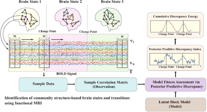
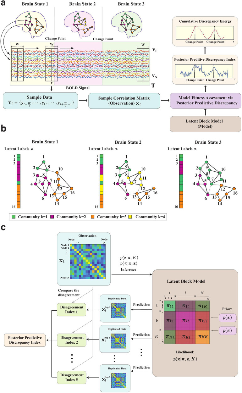
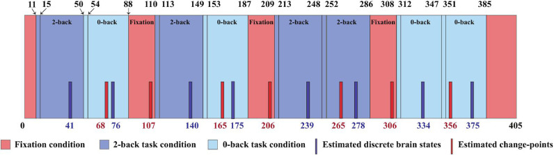
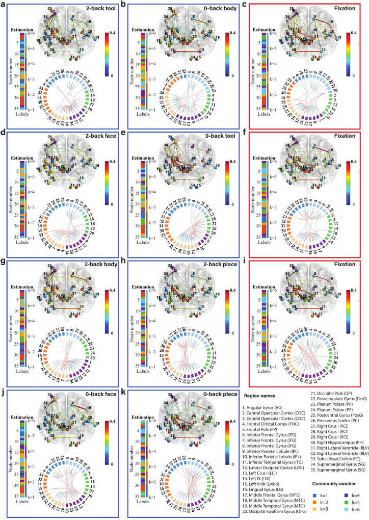
Brain function relies on a precisely coordinated and dynamic balance between the functional integration and segregation of distinct networks. Characterizing the way in which brain regions reconfigure their interactions to give rise to distinct but hidden brain states remains an open challenge. In this paper, we propose a Bayesian method for characterizing community structure-based latent brain states and showcase a novel strategy based on posterior predictive discrepancy using the latent block model to detect transitions between community structures in blood oxygen level-dependent (BOLD) time series. The set of estimated parameters in the model includes a latent label vector that assigns network nodes to communities, and also block model parameters that reflect the weighted connectivity within and between communities. Besides extensive in-silico model evaluation, we also provide empirical validation (and replication) using the Human Connectome Project (HCP) dataset of 100 healthy adults. Our results obtained through an analysis of task-fMRI data during working memory performance show appropriate lags between external task demands and change-points between brain states, with distinctive community patterns distinguishing fixation, low-demand and high-demand task conditions.

Keywords: Bayesian inference; Change-point detection; Dynamic functional connectivity; Latent block model; Markov chain Monte Carlo.

Graphical abstract

Fig. 1

The framework for identifying brain states, transitions and communities. a Schematic of the proposed Bayesian change-point detection (BCPD) method. Three different background colors represent three brain states of individual subjects with different community architectures. The colors of the nodes represent community memberships. A sliding window of width $W$ centered at $t$ is applied to the time series. The different colored time series correspond to BOLD time series for each node. The sample correlation matrix ${\mathbf{x}}_t$ (i.e., an observation for our Bayesian model) is calculated from the sample data ${\mathbf{Y}}_t$ within the sliding window. We use the Gaussian latent block model to fit the observations and evaluate goodness of fit between model and the observations to obtain the posterior predictive discrepancy index (PPDI). We then calculate the cumulative discrepancy energy (CDE) from the PPDI and use the CDE as a scoring criterion to estimate the change-points of the community architectures. b Dynamic community memberships of networks with $N$ = 16 nodes. A latent label vector $\mathbf{z}$ contains the labels ($k$) of specific communities for the nodes. Nodes of the same color are located in the same community. The dashed lines represent the (weighted) connectivity between communities and the solid lines represent the (weighted) connectivity within the communities. c Model fitness assessment. The observation is the realized adjacency matrix; different colors in the latent block model represent different blocks with the diagonal blocks representing the connectivity within a community and the off-diagonal blocks representing the connectivity between communities. To demonstrate distinct blocks of the latent block model, in this schematic we group the nodes in the same community adjacently and the communities are sorted. In reality, the labels of the nodes are mixed with respect to an adjacency matrix. The term ${\mathit{\pi }}_{kl}$ represents the model parameters in block $kl$.

Fig. 2

Effect of different levels of SNR on inter-individual variations of CDE curves. a–c CDE of the multivariate Gaussian data with SNR = 10 dB, 5 dB, and 0 dB respectively. Here, the degree of inter-individual variation (DIIV) of community structure is 0 and the dataset is simulated without HRF. The number of communities is $K$ = 6 for all of the experiments in this figure and the black plot is the group-averaged CDE curve. d–f The extrema of the individual-level CDE curves with different levels of SNR. The red dots are the local maxima and the blue dots are the local minima of 100 virtual subjects. The black plot is the group-averaged CDE curve. g The time deviation of local maxima of individual-level CDE curves compared to the local maximum of the group-averaged CDE curve with different levels of SNR. h The time deviation of local minima of individual-level CDE curves compared to the local minimum of the group-averaged CDE curve with different levels of SNR. (For interpretation of the references to color in this figure legend, the reader is referred to the web version of this article.)

Fig. 3

Results of change-point detection with different values of $K$ and local inference. a CDE of the multivariate Gaussian data with SNR = 5 dB using different models ($K$ = 6, 5, 4, and 3). The sliding window size for converting from time series to correlation matrices sequence is $W$ = 20, whereas (for smoothing) the sliding window size for converting from PPDI to CDE is $W_s$ = 10. The vertical dashed lines are the locations of the true change-points ($t$ = 20, 50, 80, 100, 130, and 160). The multi-color scatterplots in the figures are the CDEs of individual (virtual) subjects and the black curve is the group-level CDE (averaged CDE over 100 subjects). The red dots are the local maxima and the blue dots are the local minima. b Local fitting with different models (from $K$ = 3 to 18) for synthetic data (SNR = 5 dB). Different colors represent the PPDI values of different states with the true number of communities $K^{true}$. c The estimation of community constituents for SNR = 5 dB at each discrete state: $t$ = 36, 66, 91, 116, 146 for brain states 1 to 5, respectively. The estimations of the latent label vectors (Estimation) and the label vectors (True) that determine the covariance matrix in the generative model are shown as bar graphs. The strength and variation of the connectivity within and between communities are represented by the block mean and variance matrices within each panel. (For interpretation of the references to color in this figure legend, the reader is referred to the web version of this article.)

Fig. 4

Effects of DIIV and HRF on the inter-individual variations of CDE curves. a–c CDE of the multivariate Gaussian data with DIIV = 0, 5, and 10 respectively. The SNR = 5 dB and the number of communities $K$ = 6 for all experiments. d–f The extrema of the individual-level CDE curves with different levels of DIIV. The red dots are the local maxima and the blue dots are the local minima of 100 virtual subjects. g–i CDE curves of the multivariate Gaussian data applied with haemodynamic response function (HRF). j–l The extrema of the individual-level CDE curves with HRF. m The time deviation of local maxima of individual-level CDE curves compared to the local maximum of the group-averaged CDE curve with different levels of DIIV and HRF. n The time deviation of local minima of individual-level CDE curves compared to the local minimum of the group-averaged CDE curve with different levels of DIIV and HRF. (For interpretation of the references to color in this figure legend, the reader is referred to the web version of this article.)

Fig. 5

Results of local inference for the multivariate Gaussian data with HRF. a Local fitting with different models (from $K$ = 3 to 18) for synthetic data (SNR = 5 dB) with HRF. Different colors represent the PPDI values of different states with the true number of communities $K^{true}$. b The estimation of community constituents for the data with HRF at each discrete state, the centres of the state window are $t$ = 44, 74, 98, 130, 154 for brain states 1 to 5, respectively. The estimations of the latent label vectors (Estimation) and the label vectors (True) that determine the covariance matrix in the generative model are shown as colored bars. The strength and variation of the connectivity within and between communities are represented by the block mean and variance matrices within each panel.

Fig. 6

Comparison of the sensitivity of model fitness of BCPD-based states with that of block-based states using synthetic data. a Local fitting using the group-averaged adjacency matrix of BCPD-based discrete states (States 1 to 5 at time points $t$ = 44, 74, 98, 130, 154) with HRF and SNR =5 dB. b Local fitting using the group-averaged adjacency matrix of block-based states (States 1 to 5 at time points $t$ = 35, 65, 90, 115, 145) with HRF and SNR = 5 dB. c Local fitting using the group-averaged adjacency matrix of BCPD-based discrete states (States 1 to 5 at time points $t$ = 43, 75, 98, 125, 154) with HRF and SNR =10 dB. d Local fitting using the group-averaged adjacency matrix of block-based states (States 1 to 5 at time points $t$ = 35, 65, 90, 115, 145) with HRF and SNR = 10 dB. Different colors represent the PPDI values of different states with the true number of communities $K^{true}$. All experiments use the window $W_l$ = 20 for calculating the adjacency matrices.

Fig. 7

The results of BCPD for working memory tfMRI data (session 1, LR). The upper panels are the cumulative discrepancy energy (CDE) with different sliding window sizes ($W$ = 22, 26, 30, and 34; a–d under the model $K$ = 3) and different models ($K$ = 3, 4, and 5; c, e and f using a sliding window of $W$ = 30). $W_s$ is width of the sliding window used for converting from PPDI to CDE. The vertical dashed lines are the times of onset of the stimuli (which were provided in the EV.txt files in the released data). The multi-color scatter plots in the figures represent the CDEs of individual subjects and the black curve is the group-level CDE (averaged over 100 subjects). The red dots are the local maxima, which are taken to be the locations of change-points, and the blue dots are the local minima, which are used for local inference of the discrete brain states. The bottom panels show the estimated group-averaged CDE where false positives (FP) are removed using time distance threshold $\tau$ = 7. (For interpretation of the references to color in this figure legend, the reader is referred to the web version of this article.)

Fig. 8

Detected change-points and locations of the windows regarding the brain states matching the task blocks for working memory tfMRI data (session 1, LR) with $K$ = 3, and $W$ = 30. The numbers at the top of rectangles are the boundaries of the external task demands, the rectangles with background colors are the different task conditions, and the blue and red bars with specified numbers are the estimated locations of the windows for the discrete brain states and change-points. (For interpretation of the references to color in this figure legend, the reader is referred to the web version of this article.)

Fig. 9

Local fitting between averaged adjacency matrix and models from $K$ = 3 to 18. Different colors represent the PPDI values of different brain states.

Fig. 10

Community structure of the discrete brain states. The figures with blue frames represent brain states corresponding to working memory tasks (2-back tool at $t$ = 41; 0-back body at $t$ = 76; 2-back face at $t$ = 140; 0-back tool at $t$ = 175; 2-back body at $t$ = 239; 2-back place at $t$ = 278; 0-back face at $t$ = 334; and 0-back place at $t$ = 375 in a-k) and those with red frames represent brain states corresponding to fixation (fixation at $t$ = 107, 206, and 306 in c, f, and i). Each brain state shows connectivity at a sparsity level of 10%. The different colors of the labels represent community memberships. The strength of the connectivity is represented by the colors shown in the bar at the right of each frame. In Circos maps, nodes in the same community are adjacent and have the same color. Node numbers and abbreviations of the corresponding brain regions are shown around the circles. In each frame, different colors represent different community numbers. The connectivity above the sparsity level is represented by arcs. The blue links represent connectivity within communities and the red links represent connectivity between communities. (For interpretation of the references to color in this figure legend, the reader is referred to the web version of this article.)

References

1. Aicher C., Jacobs A.Z., Clauset A. Learning latent block structure in weighted networks. J. Complex Netw. 2015;3(2):221–248.
1. Allen E.A., Damaraju E., Plis S.M., Erhardt E.B., Eichele T., Calhoun V.D. Tracking whole-brain connectivity dynamics in the resting state. Cereb. Cortex. 2014;24:663–676. - PMC - PubMed
1. Aquino K.M., Fulcher B.D., Parkes L., Sabaroedin K., Fornito A. Identifying and removing widespread signal deflections from fMRI data: rethinking the global signal regression problem. NeuroImage. 2020;212:116614. - PubMed
1. Barch D.M., Burgess G.C., Harms M.P., Petersen S.E., Schlaggar B.L., Corbetta M., Glasser M.F., Curtiss S., Dixit S., Feldt C., Nolan D., Bryant E., Hartley T., Footer O., Bjork J.M., Poldrack R., Smith S., Johnsen-Berg H., Snyder A.Z., Van Essen D.C., for the WU-Minn HCP Consortium Function in the human connectome: task-fMRI and individual differences in behavior. NeuroImage. 2013;80:169–189. - PMC - PubMed
1. Bassett D.S., Porter M.A., Wymbs N.F., Grafton S.T., Carlson J.M., Mucha P.J. Robust detection of dynamic community structure in networks. Chaos. 2013;23:13142. - PMC - PubMed
Publication types