Conformational landscape of multidomain SMAD proteins

Abstract

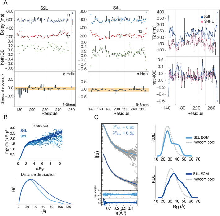
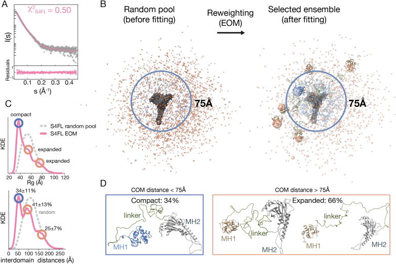
SMAD transcription factors, the main effectors of the TGFβ (transforming growth factor β) network, have a mixed architecture of globular domains and flexible linkers. Such a complicated architecture precluded the description of their full-length (FL) structure for many years. In this study, we unravel the structures of SMAD4 and SMAD2 proteins through an integrative approach combining Small-angle X-ray scattering, Nuclear Magnetic Resonance spectroscopy, X-ray, and computational modeling. We show that both proteins populate ensembles of conformations, with the globular domains tethered by disordered and flexible linkers, which defines a new dimension of regulation. The flexibility of the linkers facilitates DNA and protein binding and modulates the protein structure. Yet, SMAD4FL is monomeric, whereas SMAD2FL is in different monomer-dimer-trimer states, driven by interactions of the MH2 domains. Dimers are present regardless of the SMAD2FL activation state and concentration. Finally, we propose that SMAD2FL dimers are key building blocks for the quaternary structures of SMAD complexes.

Keywords: Intrinsically disordered regions; Multi-domain proteins; SMAD; TGFβ signaling; Transcription factor.

Graphical abstract

Fig. 1

Construct design and general workflow a. S4 and S2 domain composition. Detailed boundaries are shown in Supplementary Fig. S1A,B. b General methodology and the ensemble selection protocol. Models of the full-length proteins were prepared, including monomers, dimers, and trimers. Flexibility of the linkers was verified by NMR. Final models were selected by fitting the generated ensemble to the SAXS data using the EOM pipeline. S4FL models were validated using IM-MS data. Final ensembles were represented using the MH2 as reference (surface representation), with MH1 domains centers-of-mass illustrated as spheres of a diameter that was proportional to the frequency of a given inter-domain position within the ensemble. Linkers have been omitted for clarity.

Fig. 2

SAXS and NMR data of inter-domain linkers in solution. a S2L and S4L relaxation experiments and secondary structure propensities. The comparison of the spin–spin relaxation time, T2, and the hetNOE for S4FL and S4L. Structural propensities were calculated using ncSPC 50. The colored bar depicts the random-coil threshold and values above or below the bar represent secondary structure propensities (ɑ-helix or β-sheet/extended, respectively). For IDPs, values close to β-sheet propensity imply that these IDPs have an elongated structure. The ¹H-¹⁵N HSQC spectra showing the narrow ¹H chemical shift dispersion characteristic of IDPs is shown as Supplementary Fig. S2B. b Kratky plots for S4L and S2L are shown in dark and light blue, respectively. The high flexibility of both linkers is observed as a monotonic increase along with high s values. Distance distributions derived from the SAXS experimental profiles for S2L and S4L. The color code is the same as for the previous panel. c The experimental SAXS profiles and KDE for Rg distribution for S4L and S2L (in gray) and the solid line simulated curves from each EOM with residuals represented below. (For interpretation of the references to color in this figure legend, the reader is referred to the web version of this article.) (For interpretation of the references to color in this figure legend, the reader is referred to the web version of this article.)

Fig. 3

S4 and S2MH2 domains in solution. a Available crystal structures of S4MH2 domain. Missing residues in the electron density maps are indicated in the structure as dashed lines and as white boxes on the schematic sequence representation (on top). b SAXS scattering curve of S4MH2, corresponding to a merged curve generated from data at several protein concentrations. Residuals showing the agreement between the simulated and experimental profiles are given below the curve. Explicit models satisfying these curves are shown next to the SAXS curve. Green regions in the S4MH2 ensemble depict NMR-supported secondary structures, which were not observed in X-ray structures. c SAXS data corresponding to the S2LMH2 non-phosphorylated domain at two concentrations. In these cases, monomers (M), dimers (D), and trimers (T) (at low concentration), or only trimers (high concentration), contribute to the ensemble of conformations in solution. We provide the Kernel Density Estimation (KDE) calculated for each EOM ensemble compared to that obtained using the starting random pool of models (gray). Explicit models satisfying the curves are shown. d As in c, for S4LMH2. (For interpretation of the references to color in this figure legend, the reader is referred to the web version of this article.) (For interpretation of the references to color in this figure legend, the reader is referred to the web version of this article.)

Fig. 4

S4FL conformational landscape in solution. a The SAXS EOM simulated profile corresponding to S4FL is shown in pink. It is overlaid with the experimental profile in gray and the respective residuals are represented at the bottom panel. b EOM and random pool S4FL conformational landscapes containing 10 000 conformations. To visualize the domains in the ensemble, the MH2 domain is depicted as a surface (gray) and was used as the reference to fit all conformers. On the contrary, the MH1 domain is simplified as a sphere whose radius is proportional to the probability of occurrence for a given conformation. Large spheres that represent highly populated distributions have the MH1 domain represented as a cartoon. Blue spheres represent distributions up to a distance of 75 Å between domains, and tan spheres indicate expanded conformations. Linkers have been hidden from the representation for clarity, c Size distribution of the ensemble of conformations in the random pool and after EOM selection. The distribution shows compact (34%) and expanded (66 %) conformations, respectively. d Most representative conformations are indicated as explicit models. (For interpretation of the references to color in this figure legend, the reader is referred to the web version of this article.) (For interpretation of the references to color in this figure legend, the reader is referred to the web version of this article.)

Fig. 5

S2FL equilibrium distribution in solution. a and b SAXS curves for S2FLWT or S2FLEEE at two different concentrations in gray and EOM fittings in blue and red. Next to each SAXS curve are the Kernel density contour plots for Dmax and Volume, calculated from the EOM ensembles. M, D, and T are abbreviations for monomer, dimer, and trimer species, respectively. (For interpretation of the references to color in this figure legend, the reader is referred to the web version of this article.) (For interpretation of the references to color in this figure legend, the reader is referred to the web version of this article.)

Fig. 6

S2FLWT conformational landscape in solution. Left: distribution of MH1-MH2 inter-domain distances in the pool ensembles, in comparison to those obtained after the EOM-selection. Compact structures were classified as those with inter-domain distances less than 75 Å. Right: Models derived from SAXS data at 56.1 µM are shown following a similar approximation as that used for S4FL proteins. Representative conformations (indicated with arrows) are depicted as explicit models. To facilitate the identification of monomers, dimers, and trimers, the MH2 domains are colored in purple, green, and yellow, whereas the MH1 domains are shown in red. (For interpretation of the references to color in this figure legend, the reader is referred to the web version of this article.) (For interpretation of the references to color in this figure legend, the reader is referred to the web version of this article.)

Fig. 7

Conformational landscape of S2FL phosphomimetic variant (S2FLEEE) in solution. Inter-domain distance distribution and models derived from SAXS data corresponding to this variant. The representations are prepared following the same representations as in Fig. 6 and derived from SAXS data at 28.1 µM.

Fig. 8

Cartoon describing our hypothesis on the mechanism for the hetero-trimer association of SMAD proteins. Schematic representation of the S2FL and S4FL proteins and their quaternary structures. The MH1 and MH2 domains are represented as silhouettes generated from 3D structures. Flexible connectors have been simplified and sketched as lines. The S2FL dimer can associate either with monomeric S4FL forming a hetero-trimer, or with another monomeric R-SMAD to generate homo-trimeric R-SMAD assemblies. Each monomer of S2FL is colored with a shade of blue and monomeric S4FL is shown in orange. (For interpretation of the references to color in this figure legend, the reader is referred to the web version of this article.) (For interpretation of the references to color in this figure legend, the reader is referred to the web version of this article.)

References

1. Bornberg-Bauer E., Albà M.M. Dynamics and adaptive benefits of modular protein evolution. Curr Opin Struct Biol. 2013;23(3):459–466. - PubMed
1. Heldin C.H., Miyazono K., ten Dijke P. TGF-beta signalling from cell membrane to nucleus through SMAD proteins. Nature. 1997;390:465–471. - PubMed
1. Massague J. The transforming growth factor-beta family. Annu Rev Cell Biol. 1990;6(1):597–641. - PubMed
1. Massagué J. TGFβ signalling in context. Nat Rev Mol Cell Biol. 2012;13(10):616–630. - PMC - PubMed
1. Macias M.J., Martin-Malpartida P., Massagué J. Structural determinants of SMAD function in TGF-β signaling. Trends Biochem Sci. 2015;40(6):296–308. - PMC - PubMed
LinkOut - more resources