A metabolic modeling platform for the computation of microbial ecosystems in time and space (COMETS)

Abstract

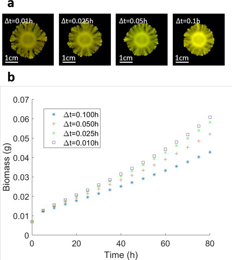
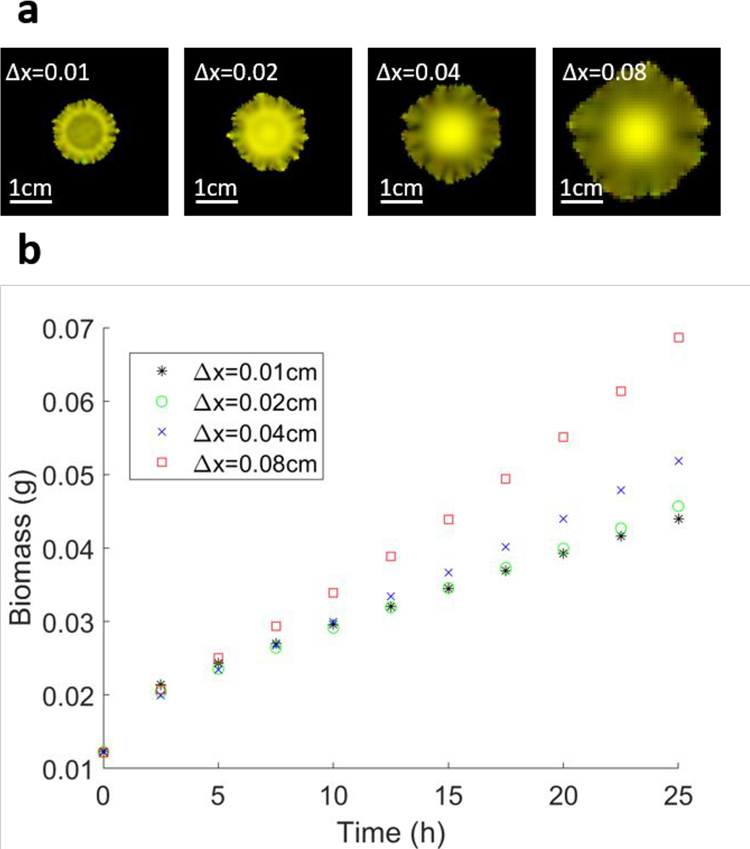
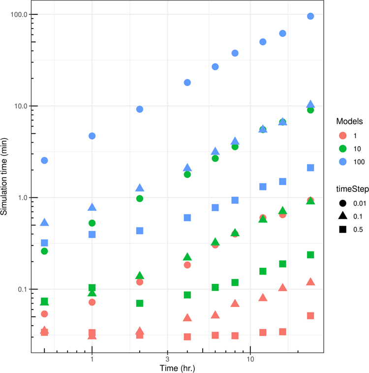
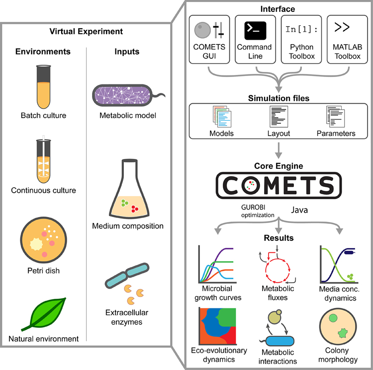
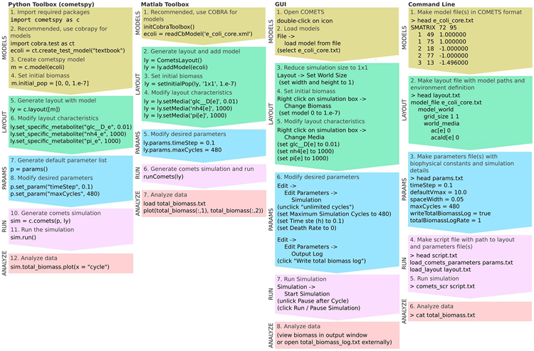
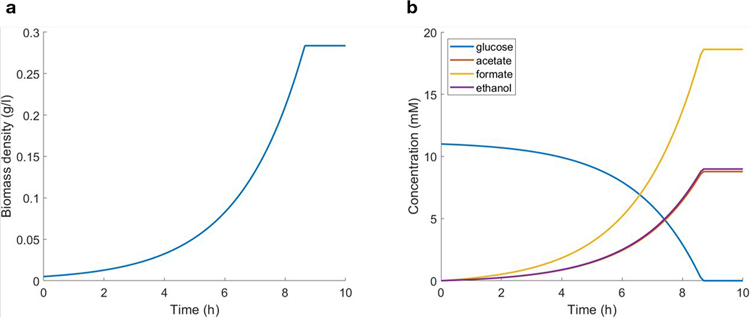
Genome-scale stoichiometric modeling of metabolism has become a standard systems biology tool for modeling cellular physiology and growth. Extensions of this approach are emerging as a valuable avenue for predicting, understanding and designing microbial communities. Computation of microbial ecosystems in time and space (COMETS) extends dynamic flux balance analysis to generate simulations of multiple microbial species in molecularly complex and spatially structured environments. Here we describe how to best use and apply the most recent version of COMETS, which incorporates a more accurate biophysical model of microbial biomass expansion upon growth, evolutionary dynamics and extracellular enzyme activity modules. In addition to a command-line option, COMETS includes user-friendly Python and MATLAB interfaces compatible with the well-established COBRA models and methods, as well as comprehensive documentation and tutorials. This protocol provides a detailed guideline for installing, testing and applying COMETS to different scenarios, generating simulations that take from a few minutes to several days to run, with broad applicability to microbial communities across biomes and scales.

Extended Data Figure 1.

Sensitivity of the simulation results depending on the value of the finite time step. Starting with a simulation identical to the one in Procedure 7, we repeated it with four different values of the time step: a) images of the final colony morphologies, b) plot of the total biomass change with time, illustrating the magnitude of the error due to the finite time step size. The simulation time step size should be chosen such that final simulation result is within the tolerated error.

Extended Data Figure 2.

Sensitivity of the simulation results depending on the value of the finite spatial grid size. Starting with a simulation identical to the one in Procedure 7, we repeated it with four different values of the grid size: a) images of the final colony morphologies, b) plot of the total biomass change with time, illustrating the magnitude of the error due to the finite grid size. The simulation finite spatial grid size should be chosen such that the final simulation result is within the tolerated error.

Extended Data Figure 3.

Sensitivity of the simulation results depending on the value of the amplitude of the demographic noise. Starting with a simulation identical to the one in Procedure 7, we repeated it with two different magnitudes of the noise amplitude $\sigma$: a) images of three replicas of a colony simulation and b) plot of the total biomass change with time of the three replicas simulations with $\sigma =0.01$; c) images of three replicas of a colony simulation and d) plot of the total biomass change with time of the three replicas simulations with $\sigma =0.01$. A finalized result of a simulation study in presence of noise should be averaged over several replicas of the stochastic simulation. The change of the noise amplitude however may have a significant effect of the growth rate and the final morphology. The value of the noise amplitude should be chosen to best represent an experimental result.

Extended Data Figure 4.

We performed a 24hr batch culture run similar to Procedure 1, with either 1, 10 or 100 models (the E. coli model iJO1366 was used in all instances). The settings were identical to Procedure 1 in the main text. We tested three timesteps, 0.01 hr. (circles), 0.1 hr. (triangles) and 0.5 hr. (squares). The x axis shows simulated time (i.e. number of simulation steps × timeStep, in hr); the y axis shows elapsed simulation time (the time taken by the computer to run the program) in min. Simulations were performed in Python using cometspy in a personal laptop running linux (Intel Core i7–10610U CPU at 1.80GHz × 4 cores, 15.3 GiB memory).

Extended Data Figure 5.

The Graphical User Interface of COMETS. COMETS simulations can be started from the GUI by loading a previously prepared layout, models and parameters files. It is meant mostly as a training tool with limited functionality. Future development of COMETS will focus on the development of a comprehensive GUI.

Figure 1.. Overview of the COMETS platform.

Virtual experiments in COMETS combine a variety of environments and biochemical inputs. These combinations can be quickly generated using one of the provided interfaces, which feed into the COMETS core engine. The engine simulates the spatio-temporal dynamics of the ecosystem and outputs microbial biomass information, metabolic fluxes, and media concentration over time. Downstream analysis, either within the toolboxes or with the user’s software of choice, can then be applied to further visualize and characterize the results.

Figure 2.

Basic workflows. Flowchart showing a typical workflow for the four interfaces for COMETS, with sufficient code / steps to run an introductory (i.e. “hello world”-like) simulation of anaerobic batch culture growth of the E. coli core model.

Figure 3.. Growth of E. coli (core model) batch culture in minimal medium, with glucose as the only carbon source.

These figures show results obtained from the simulation described in Procedure 1. a) Plot of biomass vs. time. b) Plot of the key metabolites vs. time. The biomass growth stops when the glucose is completely depleted. The production of the typical products of fermentation also coincides with the growth of the biomass.

Figure 4.. Chemostat simulation of cross-feeding E. coli strains grown on lactose.

Results from a chemostat simulation (Procedure 2), prepared with the Python toolbox, in which one strain unable to break down lactose (LCTStex_KO) receives galactose from a different strain (galE_KO) that can break lactose into glucose and galactose, but is unable to metabolize galactose. The medium environment was composed of a constant supply of lactose (lcts_e), ammonia, and trace nutrients. Galactose (gal_e) was not supplied externally but started being available in the environment as galE_KO grew. a) Biomass of the two strains over time (cycle indicates the current time step). b) Amounts of the key metabolites over time (ac_e = acetate, for_e = formate, gal_e = galactose, glyclt_e = glycolate, lcts_e = lactose, meoh_e = methanol, pppn_e = phenylpropanoate). Note that it is typical for limiting nutrients (here, lactose and galactose) to have near-zero concentrations in a chemostat. c) Fluxes of relevant exchange reactions in galE_KO, and d) LCTStex_KO (the prefix “EX_” indicates an exchange reaction, and the metabolites being exchanged with the environment are: ac_e = acetate, for_e = formate, gal_e = galactose, lcts_e = lactose, nh4_e = ammonia). Negative flux represents uptake, while positive flux is excretion.

Figure 5.. Simulations of the diurnal cycle of the marine photoautotrophic bacteria Prochlorococcus.

In this dynamic simulation of Prochlorococcus (Procedure 3), the organism is placed in an environment with a periodic light cycle, replicating the day-night alternation of sunlight. The growth of the biomass occurs only during daytime.

Figure 6.. Media concentrations over time during simulations demonstrating extracellular reactions.

Demonstration of how extracellular reactions, happening in the environment, independent of any specific organism, can be implemented in COMETS (Procedure 4). a) Environmental metabolite changes for a simple bimolecular reaction of the form A+B→C, with rate ν=νmax·[A]·[B] where νmax = 0.2 s⁻¹mM⁻¹. b) An environmental enzyme-catalyzed reaction of the form E+S→E+P, with rate according to the Michaelis-Menten equation ν=νmax·[E]·[S]/(KM+[S]), where vmax = 2 s⁻¹, KM = 0.25 mM. The enzyme E is not associated with any specific organism, and is present in the environment at a constant concentration [E]= 0.1 mM.

Figure 7.. Simulation of evolutionary processes.

In this simulation exemplifying an evolutionary process (Procedure 5), an Escherichia coli model was seeded in 1μL of glucose minimal medium (0.1mM) and transferred every 3 hours to a fresh medium using a dilution factor of 1:2 during 10 days. Mutations (in the form of reaction knock-outs) were allowed to happen in this population at a rate of 10⁻⁸ knock-outs appearing per gene and generation. The gray line represents the ancestor, which remains at high density, and other colors are used to represent different mutations that appear, persist during variable periods and extinguish stochastically.

Figure 8.. Soil-air interface simulation.

A two-species community colonizes a soil microhabitat (Procedure 6). a) Schematic detailing common features of a soil microhabitat, which are set in COMETS using simple commands to specify metabolite concentrations, and different ways of maintaining or supplementing those concentrations, in specific spatial locations. b) The initial state of the COMETS simulation, showing impenetrable barriers (gray) and the founder locations of the iJN1463 model (green) and the iYO844 model (blue). c) Time series showing biomass of the two models over time, integrated over the whole spatially structured environment. d) Snapshots of biomass and three key metabolites (f) succinate, f) O2, g) NH4) from 100 hours into the simulation. In the biomass snapshot, green is the iJN1463 model and blue is the iYO844 model. In e-g, the color scale denotes relative metabolite concentration, with bright yellow the maximum and dull purple the minimum. The scale bar shows 2mm.

Figure 9.. A variety of morphologies simulated by COMETS.

Snapshot at time 50 hours of COMETS simulations of bacterial colonies with different morphologies, implemented using the ConvNonLinDiff 2D biomass propagation model in the presence of demographic noise (Procedure 7): a) Colony of two identical strains of E. coli (labeled individually as green and red). In this case all bacterial biomass is assumed to be motile, regardless of whether or not there is growth at a given spatial location. In this case, the two strains mix, visible as yellow regions. b) Same system as panel a, except that in this case only the portions of the colony that are actively growing are assumed to be motile. In this case, the two strains are genetically demixed, forming sectors of red and green color. c) Visualization of the regions of active growth, achieved by plotting the sum of the growth rates of the two strains at individual spatial locations, for the system shown in panel a; d) Visualization of the amount of glucose left on the plate, highlighting the depletion in the area where the colony grew. The scale bar shows 1cm.

References

1. Shou W, Ram S & Vilar JMG Synthetic cooperation in engineered yeast populations. Proc. Natl. Acad. Sci. U. S. A. 104, 1877–1882 (2007). - PMC - PubMed
1. Vorholt JA, Vogel C, Carlström CI & Müller DB Establishing Causality: Opportunities of Synthetic Communities for Plant Microbiome Research. Cell Host Microbe 22, 142–155 (2017). - PubMed
1. Kehe J et al. Massively parallel screening of synthetic microbial communities. Proc. Natl. Acad. Sci. U. S. A. 116, 12804–12809 (2019). - PMC - PubMed
1. Venturelli OS et al. Deciphering microbial interactions in synthetic human gut microbiome communities. Mol. Syst. Biol. 14, e8157 (2018). - PMC - PubMed
1. Johns NI, Blazejewski T, Gomes AL & Wang HH Principles for designing synthetic microbial communities. Curr. Opin. Microbiol. 31, 146–153 (2016). - PMC - PubMed
Publication types