Image-based shading correction for narrow-FOV truncated pelvic CBCT with deep convolutional neural networks and transfer learning

Abstract

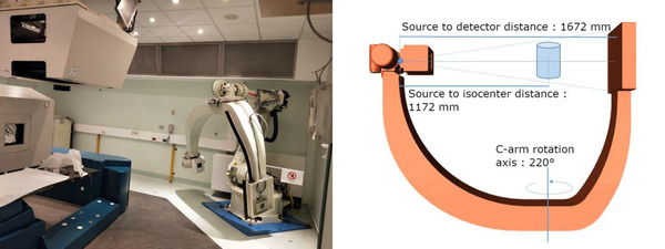
Purpose: Cone beam computed tomography (CBCT) is a standard solution for in-room image guidance for radiation therapy. It is used to evaluate and compensate for anatomopathological changes between the dose delivery plan and the fraction delivery day. CBCT is a fast and versatile solution, but it suffers from drawbacks like low contrast and requires proper calibration to derive density values. Although these limitations are even more prominent with in-room customized CBCT systems, strategies based on deep learning have shown potential in improving image quality. As such, this article presents a method based on a convolutional neural network and a novel two-step supervised training based on the transfer learning paradigm for shading correction in CBCT volumes with narrow field of view (FOV) acquired with an ad hoc in-room system.

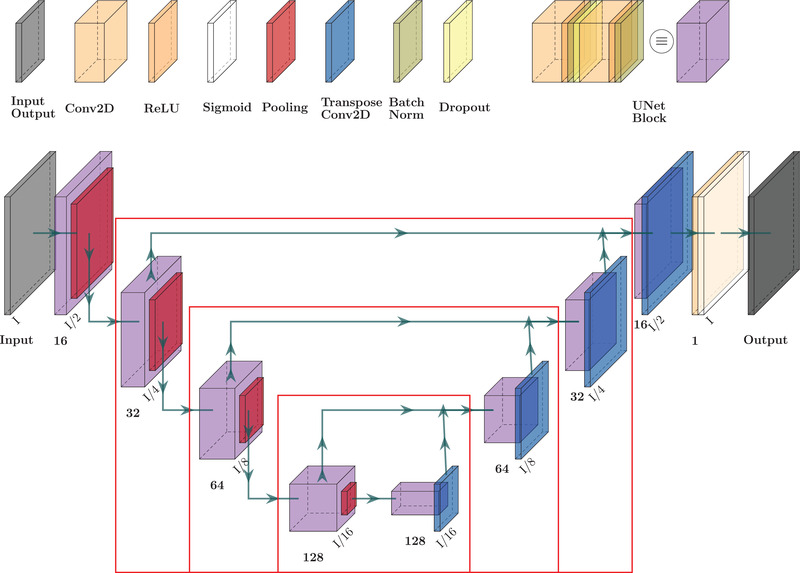
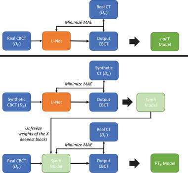
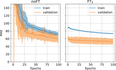
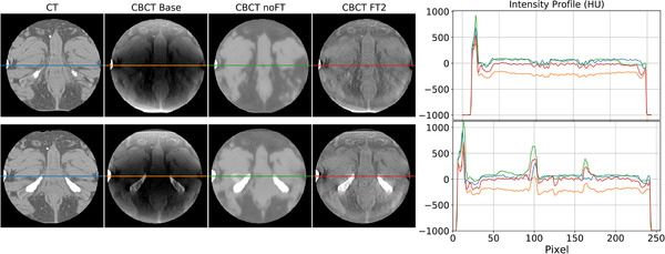
Methods: We designed a U-Net convolutional neural network, trained on axial slices of corresponding CT/CBCT couples. To improve the generalization capability of the network, we exploited two-stage learning using two distinct data sets. At first, the network weights were trained using synthetic CBCT scans generated from a public data set, and then only the deepest layers of the network were trained again with real-world clinical data to fine-tune the weights. Synthetic data were generated according to real data acquisition parameters. The network takes a single grayscale volume as input and outputs the same volume with corrected shading and improved HU values.

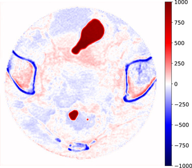
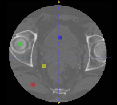
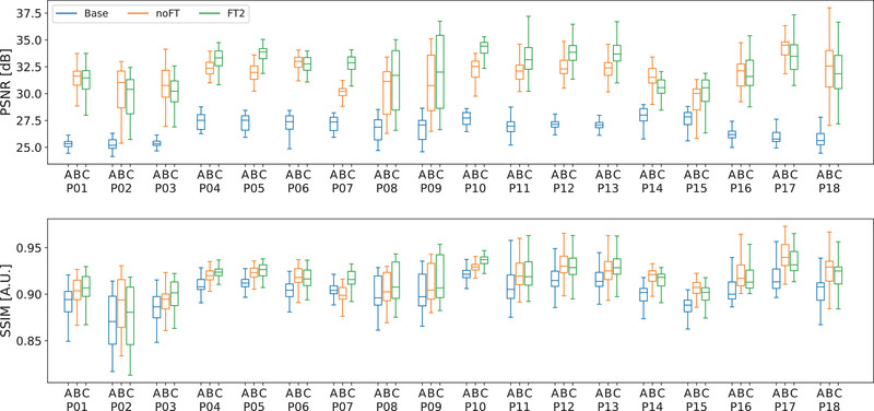
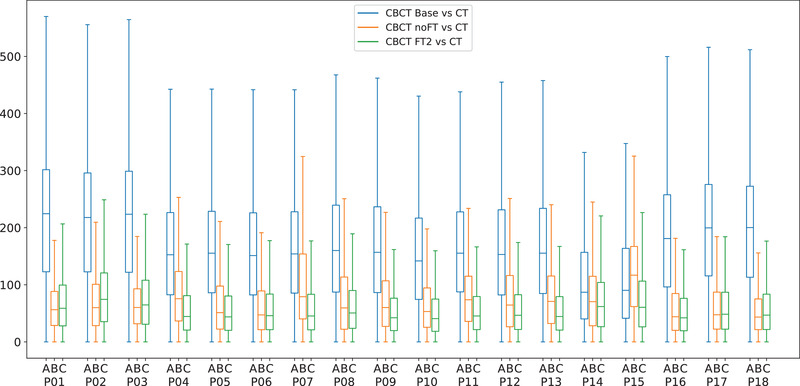
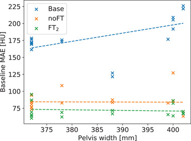
Results: Evaluation was carried out with a leave-one-out cross-validation, computed on 18 unique CT/CBCT pairs from six different patients from a real-world dataset. Comparing original CBCT to CT and improved CBCT to CT, we obtained an average improvement of 6 dB on peak signal-to-noise ratio (PSNR), +2% on structural similarity index measure (SSIM). The median interquartile range (IQR) Hounsfield unit (HU) difference between CBCT and CT improved from 161.37 (162.54) HU to 49.41 (66.70) HU. Region of interest (ROI)-based HU difference was narrowed by 75% in the spongy bone (femoral head), 89% in the bladder, 85% for fat, and 83% for muscle. The improvement in contrast-to-noise ratio for these ROIs was about 67%.

Conclusions: We demonstrated that shading correction obtaining CT-compatible data from narrow-FOV CBCTs acquired with a customized in-room system is possible. Moreover, the transfer learning approach proved particularly beneficial for such a shading correction approach.

Keywords: Hounsfield unit recovery; cone beam CT; deep learning; limited FOV; shading correction; transfer learning.

FIGURE 1

Robotic C‐arm positioned in the treatment room at CNAO. On the couch, it is possible to see a custom thermoplastic fixation mask used during the treatments (left). Schematic representation of the acquisition geometry using the aforementioned C‐arm (right)

FIGURE 2

Axial view of a D${}_r$ CBCT (left) and a D${}_s$ CBCT (right)

FIGURE 3

Schematic of the symmetric contracting and expanding paths of the U‐Net. Every U‐Net processing block (light purple) is composed of two convolutional (light orange), Relu (orange), and batch normalization (yellow) layers, with a dropout (light yellow) layer in the middle. Every block in the contracting path is followed by a max‐pooling (red) layer, while every block in the expanding path is followed by a transpose convolution (blue) one. The arrows that link two processing blocks at the same level of both paths indicate a concatenation operator. The last convolution is followed by a Sigmoid (white) layer. The red boxes indicate the blocks that can be retrained during each transfer learning experiment

FIGURE 4

Training pattern for the noFT (upper panel) and FT${}_x$ (lower panel) models. The noFT model is trained in a single step using only data from D${}_r$. The FT${}_x$ model is trained in two steps. In the first one, a model is trained using only D${}_s$ (Synth model), then only $x$ (1, 2, or 3) processing blocks were retrained with D${}_r$ data

FIGURE 5

Example of air pockets, visible as a red blob. Since these regions mismatch between the two images, corresponding voxels are not considered for HU difference computation

FIGURE 6

Example of cubic ROIs ($8\times 8\times 8$ mm) extracted from a patient. Selected regions are bladder (blue), spongy bones (green), muscle (red), and fat (yellow)

FIGURE 7

Quantitative analysis of PSNR and SSIM values between every CBCT (Base, noFT, FT${}_2$), computed for each fold of the leave‐one‐out cross‐validation

FIGURE 8

Mean absolute error history for noFT (left) and FT${}_2$ (right) models during training. Bold lines represent the mean values computed between each trained network in LOO‐CV experiments, while the shaded region represents their standard deviation

FIGURE 9

Quantitative analysis of the absolute HU difference between every CBCT (Base, noFT, FT${}_2$) and the corresponding ground‐truth CT, computed for each fold of the leave‐one‐out cross‐validation. Both models reduce the difference in the HU ranges, with better performance for the FT${}_2$ model.

FIGURE 10

Comparison between a single CBCT Base and corresponding CT axial slice with the CBCT elaborated by noFT and FT${}_2$ models. The rightmost part of the figure compares the intensity profiles of the central line of the images, highlighted by the central line in the four representations. Images are displayed with Window = 400, Level = 20

FIGURE 11

Pelvis width versus MAE for every type of CBCT (Base, noFT, FT${}_2$). MAE is calculated with respect to the CT ground‐truth

References

-
- Fattori G, Riboldi M, Pella A, et al.. Image guided particle therapy in CNAO room 2: implementation and clinical validation. Physica Medica. 2015;31:9–15. - PubMed
- Veiga C, Janssens G, Teng CL, et al.. First clinical investigation of cone beam computed tomography and deformable registration for adaptive proton therapy for lung cancer. Int J Radiat Oncol Biol Phys. 2016;95:549–559. - PubMed
- Landry G, Hua CH. Current state and future applications of radiological image guidance for particle therapy. Med Phys. 2018;45:e1086–e1095. - PubMed
MeSH terms
Grants and funding
LinkOut - more resources
Full Text Sources
Research Materials
Miscellaneous