MesoNet allows automated scaling and segmentation of mouse mesoscale cortical maps using machine learning

Abstract

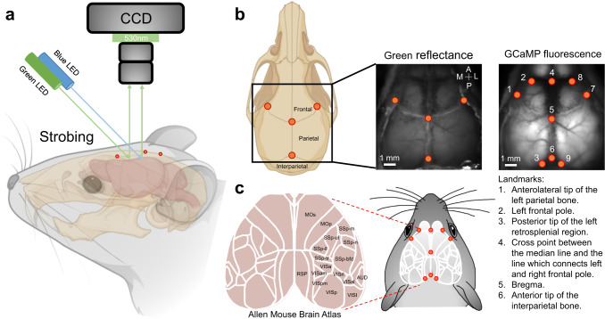
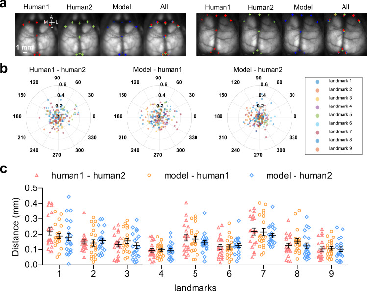
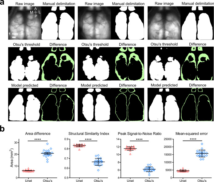
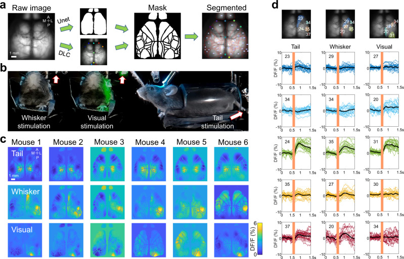
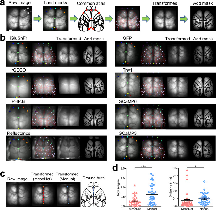
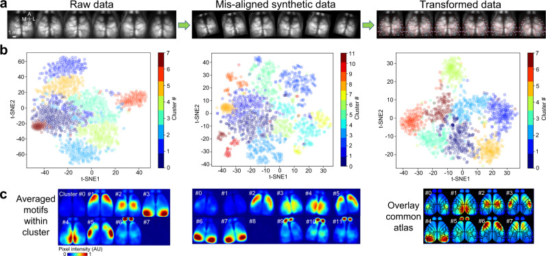
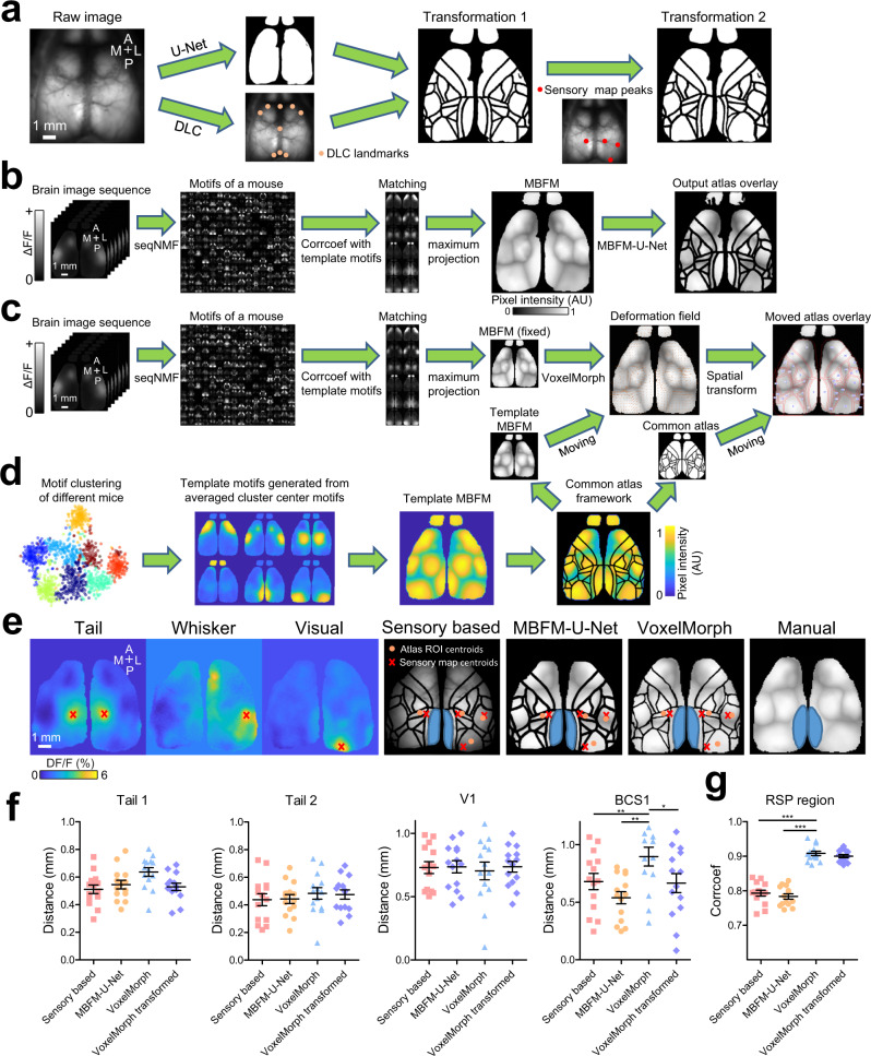
Understanding the basis of brain function requires knowledge of cortical operations over wide spatial scales and the quantitative analysis of brain activity in well-defined brain regions. Matching an anatomical atlas to brain functional data requires substantial labor and expertise. Here, we developed an automated machine learning-based registration and segmentation approach for quantitative analysis of mouse mesoscale cortical images. A deep learning model identifies nine cortical landmarks using only a single raw fluorescent image. Another fully convolutional network was adapted to delimit brain boundaries. This anatomical alignment approach was extended by adding three functional alignment approaches that use sensory maps or spatial-temporal activity motifs. We present this methodology as MesoNet, a robust and user-friendly analysis pipeline using pre-trained models to segment brain regions as defined in the Allen Mouse Brain Atlas. This Python-based toolbox can also be combined with existing methods to facilitate high-throughput data analysis.

Fig. 1. Set up of wide-field calcium imaging and definition of landmarks.

a Schematic showing green (560 nm) and blue (480 nm) LED lights targeted directly above the cranial recording window that were used to illuminate the cortex. Green reflectance and emission fluorescence were filtered using a 510–550 nm bandpass filter. The mouse head and skull were created with BioRender.com. b Examples of raw GCaMP and green reflectance images are shown with annotated landmarks. c Reference atlas (white outlines; ©2004 Allen Institute for Brain Science. Allen Mouse Brain Atlas. Available from: http://mouse.brain-map.org/) used for our segmentation process. Mop, primary motor area; Mos, secondary motor area; SSp-m, primary somatosensory area, mouth; SSp-ul, primary somatosensory area, upper limb; SSp-ll, primary somatosensory area, lower limb; SSp-n, primary somatosensory area, nose; SSp-bfd, primary somatosensory area, barrel field; SSp-tr, primary somatosensory area, trunk; VISp, primary visual area; VISa, anterior visual area; VISam, anteromedial visual area; VISpm, posteromedial visual area; VISrl, rostrolateral visual area; VISal, anterolateral visual area; VISI, lateral visual area; RSP, retrosplenial area; AUD, auditory areas.

Fig. 2. Performance of automated landmark estimation.

a Examples of model labelled and manual labelled landmarks on GCaMP images (denoted by ‘+’ symbols; blue, model labelled; red and green, manual labelled). b Polar plot of distance between coordinates of model labelled and manual labelled landmarks. c Comparison of distance between coordinates of model labelled (n = 20 mice) and manual labelled landmarks (n = 20 mice) and distance calculated by differences between coordinates of two runs of manual labelled landmarks (n = 20 mice) (scatter dot plot, line at mean with SEM, Bonferroni tests (two-sided): human1 - human2 vs model - human1, p > 0.05; human1 - human2 vs model - human2, p > 0.05; model - human1 vs. model - human2, p > 0.05; mean distance and SEM for each landmark see Supplementary Table 2). Source data are provided as a Supplementary Data file.

Fig. 3. Performance of automated delineation of brain boundary using U-Net.

a Representative images showing raw GCaMP images and respective human-applied brain delimitation as ground truth. Brain delimitation predictions from application of Otsu’s threshold (middle panel) and U-Net model segmentations (bottom panel). Green areas are the absolute differences between predicted versus ground truth. b Comparison of model-predicted (n = 20 mice) and Otsu’s threshold (n = 20 mice) brain delimitation results to ground truth by mean values for area difference (scatter dot plot, line at mean with SEM, paired t-test (two-tailed), ****p values <0.0001; U-Net, mean ± SEM = 6.11 ± 0.14; Otsu, mean ± SEM = 20.81 ± 0.73; p < 0.0001, t = 23.24), structural similarity index (U-Net, mean ± SEM = 0.83 ± 0.003; Otsu, mean ± SEM = 0.66 ± 0.01; p < 0.0001, t = 26.08), peak signal-to-noise ratio (U-Net, mean ± SEM = 11.57 ± 0.1; Otsu, mean ± SEM = 6.22 ± 0.14; p < 0.0001, t = 56.12) and mean squared error (U-Net, mean ± SEM = 4551 ± 115.9; Otsu, mean ± SEM = 15680 ± 507.7; p < 0.0001, t = 26.12). Source data are provided as a Supplementary Data file.

Fig. 4. Sensory mapping in awake mice.

a Automated alignment and segmentation pipeline of the atlas-to-brain approach. The raw GCaMP image was segmented using U-Net, and landmark estimation was done using DLC and then combined together to determine each brain region ROI. b Frontal and lateral view of an experimental set-up involving head-fixed mice with sensory stimulation cranial recording. c Sensory mapping across independent trials (n = 6 mice) shows similar regions of activation resulting from physical stimulation of the tail or whiskers and visual field of the mouse. d Single trials (n = 30 trials) of calcium temporal dynamics around the tail, whisker, and visual stimulations of different brain regions (indicated with the same colour on the brain image, the number of brain region ROIs are automatically output from MesoNet). The black line is the averaged calcium response of all the trials.

Fig. 5. Testing the brain-to-atlas approach across different lines of fluorescent protein mice.

a Automated registering and scaling pipeline of brain-to-atlas transformation (the fourth panel: big dots denote predicted landmarks on raw image, small dots denote landmarks on a common atlas, red line denote segmented brain regions; ©2004 Allen Institute for Brain Science. Allen Mouse Brain Atlas. Available from: http://mouse.brain-map.org/). b Example results of the brain-to-atlas transformation of brain image from different transgenic or virally injected mice. c Example images showing brain to atlas alignment using MesoNet or manually labelled landmarks (bregma, window margins). The performance of the alignment is based on the calculation of the distance between landmarks of anterior tip of the interparietal bone and cross point between the median line and the line which connects the left and right frontal pole, and angle of the midline compared to the ground truth common atlas, and angle of the midline compared to the ground truth common atlas (all distances and angles are reported as positive deviations compared to ground truth common atlas). d Distribution of the angle (scatter dot plot, line at mean with SEM, ***p values < 0.001, * denote p values <0.05; MesoNet, mean ± SEM = 0.28 ± 0.04; Manual, mean ± SEM = 0.62 ± 0.08; Wilcoxon signed-rank test, Two-tailed, p = 0.0005, Sum of signed ranks (W) = −446, n = 36 mice) and distance (MesoNet, mean ± SEM = 0.07 ± 0.02; Manual, mean ± SEM = 0.1 ± 0.01; Wilcoxon signed-rank test, Two-tailed, p = 0.0122, Sum of signed ranks (W) = −320, n = 36 mice). MesoNet performs significantly better in both comparisons. Source data are provided as a Supplementary Data file.

Fig. 6. Performance of brain-to-atlas transformation for clustering cortical activity motifs.

a Raw brain images, synthetic brain images, and brain-to-atlas transformed brain images from 6 GCaMP6 mice. b Scatter plot of motif clusters. An unsupervised clustering algorithm (Phenograph) was used to classify the motifs (n = 1194 motifs from 6 mice). Different colors in the t-SNE plot indicate different motif clusters. Left panel: scatter plot of motif clusters of 6 mice using raw data, silhouette score = 0.43. Middle panel: motif clusters of synthetic misaligned data, Silhouette Score = 0.39. Right panel: motif clusters of transformed data, silhouette score = 0.48. c Averaged motifs for each cluster of raw, synthetic mis-aligned, and transformed data. All the spatio-temporal motifs in each cluster were averaged, and the maximum temporal dynamics were projected onto one image. The pixel intensity scale is normalized, and the intensity value is arbitrary because responses are convolved with independently scaled temporal weightings to reconstruct the normalized DF/F fluorescence.

Fig. 7. Performance of functional sensory map and activity-motif alignment pipelines.

a Sensory map-based alignment by combining nine landmarks plus U-Net pipeline with functional sensory maps (tail, visual, and whisker stimulation-induced peak activation) to align the reference atlas to brain image. b A spontaneous activity motif matching procedure was used to generate motif-based functional map (MBFM) using calcium imaging data detected by seqNMF. The MBFM was then used to predict brain regional boundaries using MBFM based U-Net model (MBFM-U-Net). c The MBFM is used to predict a deformation field corresponding to a template MBFM using VoxelMorph. The deformation field will then be applied to the reference atlas to fit input MBFM. d The generation of template MBFM (see Methods). Different colors in t-SNE plot indicate different motif clusters. e Example images show the sensory maps and output atlas from sensory-based, MBFM-U-Net and VoxelMorph pipelines and manually painted RSP region on MBFM (blue). f Comparison of the performance of the pipelines (sensory-based, MBFM, VoxelMorph, and VoxelMorph after brain-to-atlas transformation of the MBFMs) by calculating the euclidean distance between the centroids of sensory stimulation-induced activation and predicted atlas ROIs (Tail, V1, and BCS1). Scatter dot plot, the line at mean with SEM, one-way ANOVA with Dunn’s Multiple Comparison Test. ***p < 0.001, **p < 0.01, *p < 0.05; Sensory-based vs. Voxelmorph, p < 0.05, rank = −22; MBFM-U-Net vs Voxelmorph, p < 0.05, rank = −25; VoxelMorph vs VoxelMorph transformed, p < 0.05, rank = 21, n = 14 mice). g Comparison of the performance of the pipelines (sensory-based, MBFM-U-Net, VoxelMorph and VoxelMorph after brain-to-atlas transformation) by calculating the correlation coefficient between manually painted RSP region (ground truth) and predicted RSP region by different pipelines. VoxelMorph performed significantly better than other pipelines (Sensory based vs VoxelMorph, p < 0.05, rank = −29; MBFM-U-Net vs VoxelMorph, p < 0.05, rank = −33; Sensory based vs VoxelMorph transformed, p < 0.05, rank = −23; MBFM-U-Net vs VoxelMorph transformed, p < 0.05, rank = −27, n = 14 mice). Source data are provided as a Supplementary Data file.

References

1. Petersen CCH. The functional organization of the barrel cortex. Neuron. 2007;56:339–355. doi: 10.1016/j.neuron.2007.09.017. - DOI - PubMed
1. Zhuang, J. et al. An extended retinotopic map of mouse cortex. Elife6, e18372 (2017). - PMC - PubMed
1. Gilad A, Gallero-Salas Y, Groos D, Helmchen F. Behavioral strategy determines frontal or posterior location of short-term memory in neocortex. Neuron. 2018;99:814–828. doi: 10.1016/j.neuron.2018.07.029. - DOI - PubMed
1. Cadwell CR, Bhaduri A, Mostajo-Radji MA, Keefe MG, Nowakowski TJ. Development and arealization of the cerebral cortex. Neuron. 2019;103:980–1004. doi: 10.1016/j.neuron.2019.07.009. - DOI - PMC - PubMed
1. Vanni MP, Murphy TH. Mesoscale transcranial spontaneous activity mapping in GCaMP3 transgenic mice reveals extensive reciprocal connections between areas of somatomotor cortex. J. Neurosci. 2014;34:15931–15946. doi: 10.1523/JNEUROSCI.1818-14.2014. - DOI - PMC - PubMed
Publication types
LinkOut - more resources