Convergent cross sorting for estimating dynamic coupling

Abstract

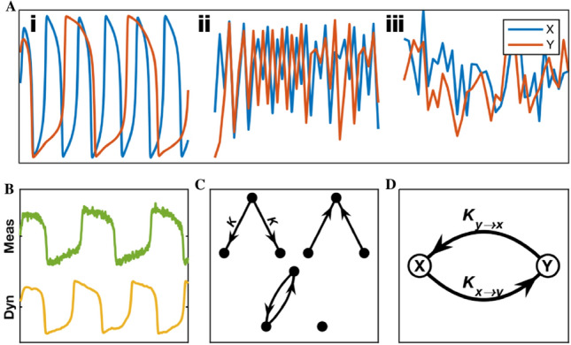
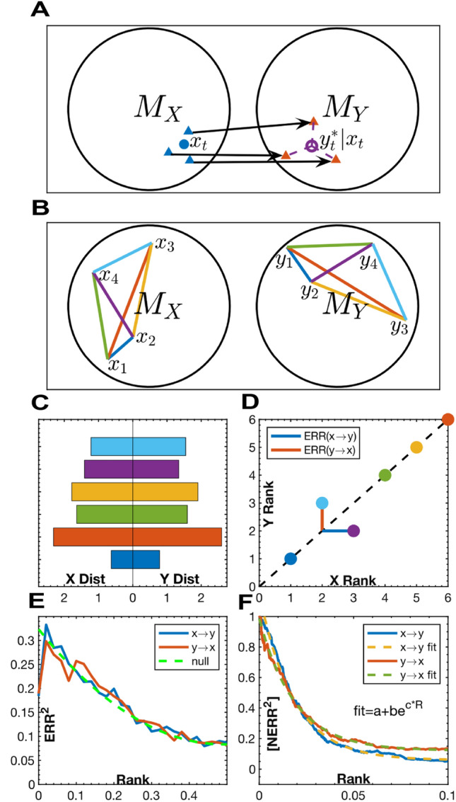
Natural systems exhibit diverse behavior generated by complex interactions between their constituent parts. To characterize these interactions, we introduce Convergent Cross Sorting (CCS), a novel algorithm based on convergent cross mapping (CCM) for estimating dynamic coupling from time series data. CCS extends CCM by using the relative ranking of distances within state-space reconstructions to improve the prior methods' performance at identifying the existence, relative strength, and directionality of coupling across a wide range of signal and noise characteristics. In particular, relative to CCM, CCS has a large performance advantage when analyzing very short time series data and data from continuous dynamical systems with synchronous behavior. This advantage allows CCS to better uncover the temporal and directional relationships within systems that undergo frequent and short-lived switches in dynamics, such as neural systems. In this paper, we validate CCS on simulated data and demonstrate its applicability to electrophysiological recordings from interacting brain regions.

Figure 1

Simulated Data. (A) Time series from the three classes of model used for validation: (i) Van der Pol Oscillators, (ii) Logistic Maps, (iii) Autoregressive Models. (B) Trace of a VDP with measurement noise (top) and (Bottom) dynamic noise. (C) Types of causal networks used to generate trials for assessing detection accuracy. Three variable networks afford the ability to test a method’s performance in the presence of third party confounds such as the common driver of two uncoupled variables in (Top Left). All other three variable topologies had to be omitted because they contain transitive causal relationships which leads to ambiguous pairwise results. In each network the coupling strength, $K$, of both edges is the same. (D) Two variable networks used to test the response to coupling parameters. $K_{x\to y}$ and $K_{y\to x}$ can vary independently.

Figure 2

The ROC AUC of CCS and CCM for detecting causal coupling in networks of three variables as a function of signal type, time series length, coupling strength, measurement noise, and dynamical noise. For each condition, the area under the curve (AUC) was calculated using 200 trials of three variable networks. (See Supplementary Area Under the Curve 3 Variable for more information on the accuracy quantification and Table S1 and Choice of Embedding Parameters for detailed methods) The shaded boundaries represent the 95% confidence intervals of the AUCs. For an additional comparison with Granger Causality see Supplementary Fig S1.

Figure 3

A comparison of CCS and CCM’s ability to determine the relative strength and directionality of coupling. (A) CCS and CCM scores for the drive from $x\to y$ as a function of the $K_{x\to y}$ and $K_{y\to x}$, signal type, $L$, SNR, and $ϵ$. $L=400$, SNR = $\infty$, and $ϵ=0$, unless otherwise specified. (B) The Spearman correlation between the true difference in coupling strength, ${(K}_{x\to y}-K_{y\to x})$ and the estimated one, $score\left(x,\to ,y\right)-score\left(y,\to ,x\right)$. (C) CCS and CCM $score\left(x,\to ,y\right)$ and $score(y\to x)$ as a function of $K_{y\to x}$ where $K_{x\to y}=0$ (i.e., unidirectional coupling). The asterisks show the points at which the means of the two distributions of scores were significantly different. The shaded regions in (B) and (C) represent 95% confidence intervals.

Figure 4

Neural experimental setup. (A) Two rats were placed in separate Plexiglas enclosures, while an implanted rat on the outside was free to roam the field and sniff through the holes in those enclosures. The implanted rats were presented with both a novel and a familiar rat. The implanted rat freely roams the field and investigates either the novel or familiar rat. Rats were removed from the field 2 min and 30 s after the onset of a trial. Trials were counterbalanced to control for place preferences, so novel and familiar rats were presented on alternating sides of the field with each trial (See SI for more info on Social Interaction Task and Animals and Housing). (B) Rats were surgically implanted with electrodes for electrophysiological recordings in the main olfactory bulb (OB), hippocampus (CA) and medial amygdala (Amg) (See SI for more details on Surgery and Neural Recordings). Figure adapted from scidraw.io under Creative Commons 4.0 license.

Figure 5

Application of CCS to multi-region neural recordings in rats. (A) Example LFP trace from a 1 s epoch. The blue, red, and green lines represent the signals from the Main Olfactory Bulb (OB), Hippocampus (Ca) and Amygdala (Amg), respectively. The time points, T1, T2, and T3 are the centers of 400 ms windows shown by the shaded regions of the plot. (B) Average 1 s CCS scores between the three regions during baseline, grooming, and sniffing behavioral epochs (See Supplementary Table S1 and Choice of Embedding Parameters for method details). The error values represent the SEM of each score. All of the scores have a significance $<{10}^{-5}$. (C) Illustration of how the CCS scores can be represented by a 6-dimensional vector. (D) The distribution of 400 ms CCS scores colored by type of behavior and plotted using the first two principal components. (E) The distribution of 400 ms CCS scores colored according to k-means cluster using five means. The inserted graphs show the network diagram corresponding to the centroid of the cluster indicated in the bottom left corner. The values in these diagrams have been corrected for the normalization and whitening transformations used for the PCA. Edges with negative values have been omitted. (F) Tables with rows showing the most frequent temporal sequences of CCS states during epochs from each of the behavioral conditions. The first three columns are the moving CCS estimates labeled and colored according to their cluster from (E). The 4th column is the percentage of epochs with that sequence. The error value is the standard error of the percentage. The 5th column is the negative log of the probability that the nth most frequent pattern would have a frequency as extreme as the one observed.

Figure 6

Illustration of Takens’ theorem. (A) A Lorenz attractor with time points colored according to proximity. (B) Time series of the $x$ coordinate. (C) Delay reconstruction from lagged $x$ coordinates. The timepoints have the same colors as those in (A). Notice how the delay reconstruction preserves the relative locations of the time points despite being transformed and warped. This demonstrates the homeomorphism between the two manifolds.

Figure 7

(A) An illustration of the CCM method. $x_t$ is point in $M_X$. The blue triangular markers represent its $D+1$ nearest neighbors where $D$ is the embedding dimension. The arrows show the mapping of each neighbor in $M_X$ to its location in $M_Y$. ${y_{\mathit{t}}}^{\mathbf{\ast }}|x_t$ is the estimate of the point $y_t$ from exponentially weighted average cross mapped neighbors from $x_t$. $CCM\left(y,\to ,x\right)=corr\left({y_{\mathit{t}}}^{\mathbf{\ast }},,,y_t\right)$ (B–F) An illustration of the CCS method. (B) Pairwise distances between the same four timepoints in $M_X$ and $M_Y$ colored according to which time points they span. (C) The magnitude of the distances in both manifolds. (D) The rank of each distance in $M_X$, $R_X$, plotted against its rank in $M_Y$,$R_Y$. The black dashed line represents perfect correspondence. The blue and red lines show the error between ranks, $ERR=$ $R_X$-$R_Y$, as a function of $R_Y$ and $R_X$, respectively. $ERR\left(x,\to ,y\right)=ERR\left(R_Y\right)$ and $ERR\left(y,\to ,x\right)=ERR\left(R_X\right)$ because they measure how well ranks in the manifold of the driven variable predict ranks in the manifold of the driver. (E) ${\mathit{ERR}}^2$ as a function of rank for a bidirectionally coupled logistic map. The ranks have been normalized between 0 and 1. The dashed green line represents the null expected ${\mathit{ERR}}^2$ for uncorrelated ranks. (F) The cumulative average of the normalized error, $\left[N,{\mathit{ERR}}^2\right],$ as a function of rank, for the system shown in (E). ${\mathit{NERR}}^2=(null-{\mathit{ERR}}^2)/null$. $\left[N,{\mathit{ERR}}^2\right]$ is thresholded at a maximum rank and fit to an exponential curve. The CCS scores are given by the y-intercepts of the fitted curves. Extrapolating from the best fit curve improves the estimate of the local correspondence by leveraging information from larger scales to overcome the high variance in ${\mathit{NERR}}^2$ observed at very low ranks.

References

1. Sugihara G, May R, Ye H, Hsieh CH, Deyle E, Fogarty M, Munch S. Detecting causality in complex ecosystems. Science. 2012;338(6106):496–500. doi: 10.1126/science.1227079. - DOI - PubMed
1. Ma H, Aihara K, Chen L. Detecting causality from nonlinear dynamics with short-term time series. Sci. Rep. 2015;4:7464. doi: 10.1038/srep07464. - DOI - PMC - PubMed
1. Quyen MLV, Martinerie J, Adam C, Varela FJ. Nonlinear analyses of interictal EEG map the brain interdependences in human focal epilepsy. Physica D. 1999;127:250–266. doi: 10.1016/S0167-2789(98)00258-9. - DOI
1. Hlaváčková-Schindler K, Paluš M, Vejmelka M, Bhattacharya J. Causality detection based on information-theoretic approaches in time series analysis. Phys. Rep. 2007;441:1–46. doi: 10.1016/j.physrep.2006.12.004. - DOI
1. Chicharro D, Andrzejak RG. Reliable detection of directional couplings using rank statistics. Phys. Rev. E. 2009;80:026217. doi: 10.1103/PhysRevE.80.026217. - DOI - PubMed
Publication types