The orbitofrontal cortex maps future navigational goals

Abstract

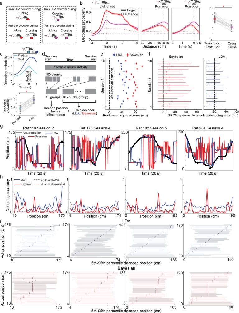
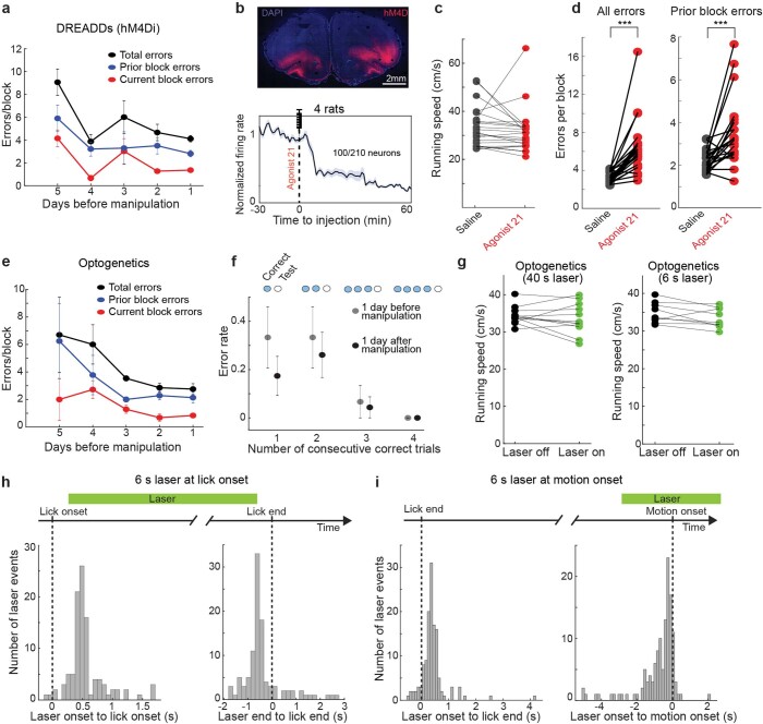
Accurate navigation to a desired goal requires consecutive estimates of spatial relationships between the current position and future destination throughout the journey. Although neurons in the hippocampal formation can represent the position of an animal as well as its nearby trajectories^1-7, their role in determining the destination of the animal has been questioned^8,9. It is, thus, unclear whether the brain can possess a precise estimate of target location during active environmental exploration. Here we describe neurons in the rat orbitofrontal cortex (OFC) that form spatial representations persistently pointing to the subsequent goal destination of an animal throughout navigation. This destination coding emerges before the onset of navigation, without direct sensory access to a distal goal, and even predicts the incorrect destination of an animal at the beginning of an error trial. Goal representations in the OFC are maintained by destination-specific neural ensemble dynamics, and their brief perturbation at the onset of a journey led to a navigational error. These findings suggest that the OFC is part of the internal goal map of the brain, enabling animals to navigate precisely to a chosen destination that is beyond the range of sensory perception.

Fig. 1. Goal-specific firing of OFC neurons.

a, Schematic of the task. b, Firing of two representative neurons showing spike rasters and rates over position with two running directions in black and grey (left) or over time from lick onset (right). c, Firing across trial blocks during running (speed >10 cm s⁻¹) or licking. d, Left, well-dependent firing across trial blocks. Middle and right, invariant firing to the difference in running direction (middle) or starting well (right). e, Colour-coded rate plots along the position and navigation phase of the animal. Shown are all rewarded wells approached in the direction of the higher activity of the neuron. f, Distribution of peak firing along navigation phase for all OFC neurons encoding position and navigation phase. *Outlier by generalized extreme studentized deviate test (above the threshold of 607.22 neurons at P = 0.05). g, Pie charts showing the numbers of neurons with spatial and/or navigation phase tuning. h, Left, decoding of licking well (target) and other wells (other). Middle, decoding of run-over well against distance (left) and time (right). Right, comparison of decoding between licking and run-over well, showing individual 18 sessions (grey) and means (red). *P = 1.96 × 10⁻⁴ in two-sided Wilcoxon signed-rank test. i, Decoding of licking well when the corresponding approach direction was excluded from the training of the decoder (left) or when all trials from the corresponding goal well pair were excluded from the training of the decoder (right). In c, d, h and i, plots show mean (line) ± s.e.m. (shaded).

Fig. 2. Persistent goal representation in the OFC.

a, Firing of two representative neurons aligned to motion onset (MO) and lick onset (LO) or throughout navigation on normalized time (right). b, Same as a, except that the plots are based on ensemble neural activity projected on the axis with maximum goal well separability. c, Two representative trials showing the position of the animal (black) and the decoded well (red; well with maximum decoding probability). d, Decoding of goal well (blue) and current well (red), together with the wells next to current goal (magenta) or before goal (cyan), plotted over time from motion onset (left) or positional fraction of journey (right). The inset on the top left shows the displacement of the animal’s position. n = 18 sessions. e, Plot shows the times at which the decoding probability of the goal well first exceeded that of the current well. n = 18 sessions. f, Decoding of the goal well (as in d) compared to chance levels calculated on five null hypotheses (see Methods). In a, b, d and f, plots show mean (line) ± s.e.m. (shaded). AU, arbitrary units.

Fig. 3. Orthogonal coding of spatial goals to evolving OFC dynamics.

a, Illustration of dynamic coding. Left, firing of three neurons aligned to motion onset. Right, firing of the same neurons plotted on individual axes of a three-dimensional space, forming similarly shaped activity trajectories separated from each other depending on future goals. b, Ensemble activity of OFC neurons in reduced dimensions using PCA plotted separately aligned to motion and subsequent lick onsets (left) or in normalized time (right). Shown are trial averages based on goal wells. c, Ensemble neural activity in individual trials projected on the axes with maximal goal well separability using LDA, calculated at individual time points and reduced to two dimensions using Isomap. Opaque circles with error bars denote mean ± s.e.m for each well. d, Relationship between the evolution of dynamics and the goal well separability. Top, as in a, along with the axis of maximum well separability (first LDA dimension). Instantaneous velocities of neural trajectories are shown with arrows. Bottom, plot shows angular differences (in degrees) between the velocity vectors and the major LDA axis from individual 18 sessions (thin) and means (thick). e, Plot shows three principal components (PCs) of neural activity trajectories from individual trials extracted using LDA (Methods). Left, original trajectories from neural data, separately aligned to motion onsets (thin) and lick onsets (thick). Right, simulated trajectories from the first-order linear dynamic model fed with neural activity at motion onset. f, Top, goal decoding from the real (original) and the simulated (model) trajectories. Bottom, destination decoding between correct and error trials from the simulated trajectories. Dashed lines indicate chance levels. In a and f, plots show mean (line) ± s.e.m (shaded). n = 18 sessions. AU, arbitrary units.

Fig. 4. OFC perturbation impairs accurate navigation.

a, Top, coronal section showing expression of bReaCh-ES-eYFP (green). Dotted white lines indicate the positions of optic fibres. Bottom, plot shows spike rasters and mean rates of a representative OFC neuron during a 6-s laser pulse train (15-ms pulses at 5 Hz). n = 14 trials. Scale bar, 2 mm. b, Plot shows a representative behaviour of the bReaCh-ES-expressing animal. The position of the animal is plotted over time (black line), together with the licking of the animal at either correct (blue) or incorrect (red) wells. Previous block errors are shown with arrows. c, Error rates of the animals before, during and after a 40-s laser pulse train (mean ± s.e.m.). Errors to the wells rewarded in the previous block are shown separately. **P < 0.01 or *P < 0.05 in two-sided Wilcoxon signed-rank test with post hoc Bonferroni correction. n = 12 sessions from three rats. d, Error rates of the animals subjected to a 6-s laser pulse train applied at motion onset (black) or lick onset (grey). Error bars denote s.e.m. n = 9 sessions from three rats. *P = 0.020 or **P = 0.008 in two-sided Wilcoxon signed-rank test.

Extended Data Fig. 1. Behavioural performance in the navigation task.

a, Top view photo of the linear maze used in this study. b, Mean number of errors committed per trial block during the first 15 days of training. Prior block errors are defined as incorrect licking of wells that were rewarded in the previous block. Current block errors are defined as incorrect licks of the same well from which the animal obtains its most recent reward in the block (by failing to visit its paired well). Topological errors comprise incorrect licks of the wells immediately next to the correct target well (but if this erroneously licked well was rewarded in the previous block, it was classified as prior block error.) The near absence of topological errors implies that animals form a robust spatial map that enables accurate estimation of well positions. c, Mean number of successfully completed blocks per session. As the animals learned the task, block transitions occurred quicker, resulting in a steady increase in the number of successfully completed blocks before saturating after 8 days of training. In panels b-c, n = 5 rats for days 1–12, 4 rats for day 13, and 3 rats for days 14-15. d, Average error rates after consecutive correct licks. Numbers in the horizontal axis indicate the number of consecutive correct licks prior to the trial being evaluated (as shown in the schematic on top where blue circles denote correct trials and white circles represent the trial whose outcome was analysed. Data are plotted separately for different stages of training. After five and six consecutive correct trials, the probability of making an error in the subsequent trial was reduced to 6.86% and 8.32%, respectively, and was not significantly different across different stages of training (p = 0.0261, 0.0006, 0.0416, 0.0476, 0.2074, and 0.0911 in 1-way ANOVA for error rates following 1-6 consecutive correct trials, respectively; n = 5 rats). We thus introduced a block change of well combinations only after the animal made at least six consecutive correct trials. e, Prior block errors were not purely due to the animal’s habitual behaviour. We analysed trials in which the same well was rewarded in both previous and current blocks (well A in the scheme) and its paired well in the previous block (well B in the scheme) was in the middle of journey toward the other goal well in the current block (well C in the scheme). The average number of prior block errors in the trained animals proportionally increased as the distance between well B and well C reduced. Dotted line represents the best fit linear regression line (slope: 0.206, p = 0.02 from two sided t-statistic with the null hypothesis of zero slope. n = 13, 9, 6, 12 sessions from 5 rats for d = 4, 3, 2, 1, respectively). f-h, Plots showing the distributions of (f) lick durations, (g) time latencies between the end of licking and the onset of motion, and (h) entire times from lick onset to motion onset. Each distribution was further divided into two plots according to the length of lick threshold. The left plots are based on 12 sessions with the lick threshold of 2 s as well as 1 session with the threshold of 1.5 s, and the right plots are on 5 sessions with the threshold of 1 s. Dotted lines represent the medians. i, Decoding probability of the well that was approached and licked by the animal (as in Figure 1h) plotted according to different levels of lick threshold (n = 13 and 5 for the threshold of > 1 s and = 1 s, respectively). Shown are means (line) ± s.e.m (shaded). j, No significant difference in error rates between the two consecutive blocks with a common goal well and those without it. Each dot represents the mean from an individual session (p = 0.08 in two-sided Wilcoxon signed-rank test; n = 18 sessions from 4 rats). Error bars in panels c, d, and e denote s.e.m.

Extended Data Fig. 2. Tetrode locations and bReaCh-ES-eYFP expression in OFC.

a, Nissl-stained coronal sections of all animals recorded from OFC (4 rats) with tetrode tracks marked with arrows. b, Coronal sections showing the expression of bReaCh-ES-eYFP (green) in bilateral OFC of the three animals used for optogenetic perturbation experiments. Dotted white lines indicate the positions of the optic fibres.

Extended Data Fig. 3. Firing properties of individual OFC neurons.

a, Procedure for quantifying spatial selectivity (see Methods) of OFC neurons. Colour coded firing rates during 200 pseudotrials and their shuffled counterparts are shown in top and middle panels, respectively. First 100 pseudotrials are during stationary periods (speed < 10 cm/s) and the next 100 are during periods of motion (speed > 10 cm/s). Panel on bottom shows the distributions of mean spatial correlations obtained from 1000 original (light grey) and shuffled (dark grey) sets of pseudotrials for this neuron. b, Top: three representative neurons that conjunctively encode spatial location and navigation phase. Bottom: three examples of spatially selective neurons that were not influenced by navigation phases. Same convention as in Figure 1e. c, Cumulative frequency of spatial information calculated over firing rates in a 2D space of position × navigation phase (as in b) versus that taking into account only positional differences (and hence averaged across phases) for all 2056 neurons representing position and navigation phase conjunctively. Spatial information in the conjunctive position × phase space is greater than the one considering positional differences only (p = 1.78 × 10⁻¹⁸⁰ in two-sided Wilcoxon ranksum test). d, Peak firing rate of 10 representative neurons during licking. Single dots represent individual trials, and the well identity is colour coded. p-values calculated using one-way ANOVA. e, Well-specific but paired-well-independent firing rate of four representative neurons (one from each animal). Same convention as in Figure 1d. f, Peak firing rate of 10 representative neurons during −0.5 to 0.5 seconds relative to motion onset. Single dots represent individual trials and are coloured based on the identity of goal well. p-values calculated using one-way ANOVA. g, Four representative neurons with goal-well dependent but start-well independent firing at motion onset. p-values calculated using one-way ANOVA. h, Session-based summary of the numbers of neurons categorized as active (average firing rate > 0.5), current-well selective, and goal-well selectivite (see Methods), together with the number of dimensions explaining 85% of the variance of goal-selective neurons (obtained using PCA). i, Total numbers of active neurons (average firing rate > 0.5 Hz) during each of the following behavioural phases; running, approach (duration of 500 ms prior to lick onset), and well-licking. j, Firing rate plots of the same representative neurons as in Figure 2a with trials averaged (and coloured) based on ‘current’ well. In panels e and g, plots show means (line) ± s.e.m. (shaded).

Extended Data Fig. 4. Low spatial information in OFC neurons.

a-b, Colour-coded firing rate plots of representative OFC neurons and CA1 neurons during a random foraging task in an open-field arena. c, Top: spatial information of individual OFC and CA1 neurons in the random foraging task. Error bars denote s.e.m. Inset shows the distribution of spatial information of the OFC and CA1 neurons. ***p = 5.76 × 10⁻²⁰, z = 9.14 in two-sided Wilcoxon rank-sum test. Bottom: distribution of spatial information of individual OFC neurons during the goal-directed navigation task on the linear maze. Solid and dashed vertical lines indicate the median and mean, respectively. d, Stability of spatial tuning during the session. Top: rate maps of two representative neurons, each from OFC and CA1, during the first and second halves of the session. Bottom: histogram of spatial correlations of 70 OFC neurons and 65 CA1 neurons. For each neuron, rate maps were calculated separately for the first and second halves of the foraging sessions, and the correlation between the two position-dependent firing-rate vectors was evaluated (spatial correlation: OFC, 0.19 ± 0.02, CA1, 0.79 ± 0.02; two-sided Wilcoxon rank-sum test: z = 9.72, p = 2.45 × 10⁻²²).

Extended Data Fig. 5. Validation of goal-well decoding.

a, Decoding of goal well (blue), current well (red), and previous well (green), in the trials where the animal’s next goal and previously-visited well were different due to error trials. n = 18 sessions. MO: motion onset. b, Decoding of the wells during a 3-well task. Bottom plot shows the decoding probabilities of the wells when the animal’s next goal and the previous goal were different. The decoder indicated the animal’s next destination but not the previous goal. c, Top: decoding on error trials showing the probabilities of current well (red), the animal’s next destination visited incorrectly (green), and the correct well according to the task rule (grey), plotted over time (left) or along positional fraction (right). Bottom: decoding of the animal’s next destination at motion onset between correct (blue) and error (green) trials. Dots represent individual 18 sessions. p = 0.372 in two-sided Wilcoxon signed-rank test. d, Top: schematic of the experimental setup and the behaviour paradigm of a continuous alternation task. The correct destination of individual trials switched alternately between Goal 1 and Goal 2. For successful task performance, rats needed to follow the sequence of trajectories outlined by numbers 1 to 4. Two rats were trained with the same strategy as described before, and the performance of both rats reached over 95% accuracy. Bottom: decoding probability of goal well during navigation. Decoding was performed by using a decoder based on quadratic-discriminant analysis that was trained on OFC neural activity during the concatenated time range from −1 s to 1 s relative to motion onset (at the start well) as well as from −2 s to 2 s relative to lick onset (at the goal well). Decoding was restricted to correct trials with trajectory paths 1 and 3 in the top schematic. Each trial was decoded in a leave-one-out cross-validated manner. Decoding performance is plotted across four contiguous time phases: 1) 5 s duration prior to motion onset at the start well, 2) from motion onset to the choice point, 3) from the choice point to lick onset at the goal well, and 4) 3 s duration after lick onset. Due to trial-by-trial variability in the animal’s behaviours, the second and third phases are plotted in normalized time for each. Grey line denotes aggregate chance level from well-based and speed-based null hypotheses (see Methods; chance levels for goal distance and direction were not considered because they were identical between the two goal-directed navigations in the maze). The decoding probability of goal well was significantly greater than chance starting from 0.6 s prior to motion onset until 2.6 s after lick onset at the goal well (decoding probability at motion onset: 0.74 ± 0.06, compared to its chance level of 0.58; n = 4 sessions from 2 rats). MO: motion onset, CP: choice point, LO: lick onset at goal well. e, Schematic of chance level calculation (see Methods). All five parameters are tested for the goal-well decoding, whereas only the direction and the random well selection were considered for the current-well decoding. f, Decoding performance of goal well using the following three kinematic variables together as predictors: acceleration (calculated as in Kropff et al.), speed, and head direction (dotted line). The decoder was separately trained and tested on individual time points. The decoding performance based on the activity of OFC neurons is also included for comparison. Grey horizontal line denotes the times when the goal-decoding performance of the neuron-based decoder was significantly better than that based on kinematic variables (p < 0.05; two-sided Wilcoxon signed-rank test followed by Holm-Bonferroni correction, n = 18 sessions). g, Top: acceleration at motion onset at individual trials from a representative session plotted as a function of the distance to the goal (measured in a well-interval unit). The regression line best fitting the data is shown with the dotted line. The p-value of the regression slope is shown on top. Bottom: the regression slope between the acceleration at motion onset and the goal distance for all 18 sessions. Red asterisks denote sessions with statistically significant regression slope (p = 0.0015, 0.0065, 0.0885, 0.3239, 0.8152, 0.1810, 0.0289, 0.0024, 0.0744, 0.0087, 0.0008, 0.0025, 0.0042, 0.0717, 0.9600, 0.2889, 0.9802, 0.9101, from the t-statistic with the null hypothesis of zero slope without multiple comparison correction). h, Goal representation is largely independent of the animal’s speed or acceleration. Top left: for testing the effect of the animal’s speed at motion onset, we took an approach of grouping based on the animal’s running speed, whereby trials were divided into either two or four groups. Top right: we used the same strategy for testing the effect of the animal’s acceleration at motion onset. In both cases, we obtained almost the same chance levels between these two grouping strategies. Bottom left: goal decoding probability in trials with quick start using a decoder trained only on trials with slow start. Bottom right: data used in training and testing of a decoder were swapped. i, Decoding probabilities of ‘current’ well at different timepoints. Schematic on top depicts the time durations used for the decoder’s training (dark grey lines) with the class label of current well. Left: decoding of current well using the same strategy as used for the goal-well decoding (Figure 2d). Second left: identical to Figure 1h left but is included for comparison. Third and Fourth: decoding of current well relative to lick end and motion onset, respectively. The results together suggest that the current well is only weakly represented in OFC both at motion onset and during navigation, irrespective of the decoding strategy. MO: motion onset, LO: lick onset, LE: lick end. j, Decoding of current well as in Figure 1h, but with shorter durations of training data denoted in the schematic on top. k, Decoding probabilities and corresponding aggregate chance levels of the current (left 4 plots) or the goal (right 4 plots) well on a representative session from each rat. Same notations as in Figure 1h left or 2d left (trial number for the current or the goal well decoding: Rat 110 session 2, n = 137 and 119; Rat 175 session 5, n = 116 and 114; Rat 182 session 5, n = 149 and 146; Rat 284 session 5, n = 133 and 133). In panels a–d, f, and h–k, plots show means (line) ± s.e.m. (shaded).

Extended Data Fig. 6. Decoding of the animal’s position during motion from ensemble activity of OFC neurons.

a–b, Comparison of well representation of OFC neurons during licking versus crossing. a, Schematic of two different decoders. Left: a decoder was trained on the neural activity as animals approached and licked a target well (lick decoder). This decoder is the same as in Figure 1h. Right: another LDA-based decoder was trained on the neural activity as animals crossed a well without licking it (cross decoder). Training and testing for this cross decoder were performed in a 10-fold cross-validated manner, in which the entire session was divided into 10 equal-duration groups and the neural activity during well crossing from 9 groups were used to train a decoder, while the left-out group was used for testing. b, Left: decoding probability of licking well based on the two types of decoders trained during licking (red) or crossing (magenta). Middle two panels: distance (left) and time (right) based decoding of crossing well based on the two decoders. The red traces are identical to those in Figure 1h. Shown are means (line) ± s.e.m. (shaded). n = 18 sessions. Right: decoding probability of licking well using the decoder trained on the data during well licking, compared with that of crossing well based on the decoder trained on the data during well crossing. Results from individual sessions are shown in small grey circles while larger circles with error bars denote means ± s.d. (decoding probability of licking well: 0.67 ± 0.07; crossing well: 0.41 ± 0.08; *p = 1.96 × 10⁻⁴ in two-sided Wilcoxon signed-rank test), suggesting that well representation of OFC neural population is particularly strong during licking at goal wells. c, Top: decoding probabilities of goal well and its immediately preceding ‘pre-goal’ well when the animal crossed over the pre-goal well. The decoding of pre-goal well was performed using a decoder trained on cross-over wells (as in a–b), whereas goal-well decoding was performed by a decoder trained on a 2 s period prior to lick onset at goal wells. Shown are means (line) ± s.e.m. (shaded). Bottom: decoding probabilities of pre-goal and goal wells at the time of crossing the pre-goal well. Results from individual sessions are shown in small grey circles while larger circles with error bars denote the means ± s.d (decoding probability of pre-goal well: 0.37 ± 0.08; goal well: 0.59 ± 0.07; two-sided Wilcoxon signed-rank test: *p = 1.96 × 10⁻⁴). d, Schematic of the strategy to decode the animal’s instantaneous position from OFC neural population activity. As the animal perform multiple trial types with various start and goal positions during a session, the entire time duration of the session was first divided into 100 chunks of equal duration, and 10 groups were created by sampling 10 chunks per group randomly (without repetition), which ensure unbiased distributions of spatial bins among groups. To decode the spatial location, we then divided the animal’s position along the linear maze into 5 cm spatial bins. Spatial decoding was carried out on each group using 10-fold cross-validation, in which the neural activity during motion (speed > 10 cm/s) from 9 out of 10 groups was used to train a decoder while that of the left-out group was used for prediction of the rat’s location. Two types of decoding algorithms – LDA and Bayesian – were implemented. For LDA-based decoding, we trained a regularized LDA decoder (see Methods) with ensemble firing rate vectors at individual 100 ms bins using the class label of spatial bin occupied by the animal. For Bayesian decoding, we first calculated mean firing rates of each neuron at individual positions, and then estimated the posterior probability of the animal’s position at a particular spatial bin in a 100 ms bin using the following formula, $P\left(b_k\right)=C\left({\prod }_{i=1}^N\right(b_k^{i}f\left){}^{s_i}\right)e^{{-\sum }_{i=1}^N{b}_k^{i}f}$. where $b_k$ is the k^th spatial bin, C is a normalizing constant, N is the number of neurons, $b_k^{i}f$ is the average firing rate of the i^th neuron at the k^th spatial bin (calculated as the average number of spikes per 100 ms), and $s_i$ is the number of spikes fired by the i^th neuron during a given time bin. For both decoding strategies, the spatial bin with the highest probability was assigned as the decoded position. The decoders were trained on the activity of all neurons with mean firing rates greater than 0.5 Hz. e, Root mean squared decoding error for each session using the two decoding strategies (average root mean squared error for LDA and Bayesian: 39.51 ± 1.06 cm and 56.41 ± 1.49 cm respectively compared to the well spacing of 20 cm shown in a dotted vertical line; n = 18 sessions). f, Distribution of absolute decoding errors resulting from Bayesian (left) and LDA based (right) position decoding, shown as thin horizontal lines ranging from 25th to 75th percentile with ticks denoting the median. Each line represents data from one session. g, Decoded positions (vertical axis) during a 20 second period (horizontal axis) from four representative sessions. Positions decoded using LDA and Bayesian are shown in blue and red, respectively. h, Mean decoding accuracy, defined as a fraction of correctly decoded positions, for every spatial bin from representative sessions. Chance levels for LDA decoders were obtained by shuffling class labels during the decoder’s training. This procedure was repeated 100 times, generating a distribution of mean accuracies across spatial bins. Chance level for each bin was set at 95th percentile of this distribution. Similarly, for Bayesian decoding, chance levels were assessed based on shuffled firing rates among spatial bins. i, Distribution of decoded positions, shown as thin horizontal lines ranging from 5th to 95th percentile with ticks denoting the median, against the actual spatial location (vertical axis) occupied by the animal. Plots show the results of 4 representative sessions with a decoding strategy based on either LDA (top row) or Bayesian (bottom row).

Extended Data Fig. 7. Choices of hyperparameters, decoding algorithm, and data range to optimize the goal decoding.

a, Illustration of the impact of dimensionality reduction on goal-well decoding. This strategy, as well as the followings (b and c), were aimed to reduce the decoder’s dimensionality, as a decoder with a large number of parameters results in poor performance on a test dataset in general. Shown in each plot are the mean goal decoding probability and the corresponding chance level based on the data from a representative session (top) or across all sessions (bottom) (see Methods and Extended Data Fig. 5 for details). We implemented PCA to reduce the data dimensions to different degrees of explained data variance, and assessed the impact of dimensionality reduction on the performance of goal-well decoding. The decoding performance was optimal when the number of chosen dimensions explained 85% of the data variance, in terms of the maximum separation from the corresponding chance level as well as a small variance of the decoding probability. The decodings were performed with a fixed regularization value of 0.5 on goal-well selective neurons. b, Illustration of the impact of regularization. Shown are the decoding performances at three levels of regularization values. We found that the regularizer value of 0.5 has the maximum separation from the corresponding chance level as well as a low variance of the decoding probability. The decodings were performed with reduced dimensions explaining 85% of the data variance on goal-well selective neurons. c, Illustration of the impact of pre-selection of goal-well selective neurons. The decoding performance was assessed based on either goal-well selective neurons (left) or all recorded neurons (right). We found that the pre-selection of goal-selective cells achieved better separation from the corresponding chance level. The decoding was performed with the reduced dimensions explaining 85% of the data variance and the regularization value set to 0.5. d, Plots show a summary of decoding performance at motion onset relative to the corresponding chance level using different parameters described in a–c. *p < 0.05, **p < 0.01, and ns (p > 0.05). Left: p = 0.0936, 0.0156, 0.0084, and 0.9479; Middle: p = 0.0429, 0.0139, 0.0096, 0.0065, and 0.0279. Right: p = 0.0084, and 0.3061; in two-sided Wilcoxon signed-rank test without multiple comparison correction. n = 18 sessions. Errorbars denote s.e.m.). e, Comparison of decoding performance of goal well between two algorithms, LDA (left) and a support vector machine (SVM, right). For SVM we used a box-constraint of 0.01. Plotted are the decoding accuracy of goal well. For LDA, the predicted well was chosen as the one with the maximum probability. The two algorithms achieved similar decoding performance (the mean accuracy relative to the chance level at motion onset: LDA 0.0365; SVM 0.0432). f, Left: performance of decoders trained with different time ranges of neural activity. Four different ranges of the data were used as illustrated on top of each plot (orange bars). We found that the goal decoding improved by concatenating the neural activity at both motion onset and lick onset. Furthermore, the decoding performance at motion onset improved as a longer time range of the data was used for the decoder’s training. Interval 3 is the same as in Figure 2d. Right: summary of decoding performance at motion onset relative to the corresponding chance level for the four different decoding strategies described in left panel (n = 18 sessions, errorbars: s.e.m.). *p < 0.05, **p < 0.01, and ns (p > 0.05). p = 0.0176, 0.0642, 0.0084, and 0.0016 in two-sided Wilcoxon signed-rank test without multiple comparison correction. g, Plots showing the times when the decoding probability of the goal well exceeded that of the current well for each of the decoding strategies shown in panel (f) above. Grey diamonds indicate data from individual sessions (n = 18 sessions). Light vertical dotted line denotes the mean across sessions (interval 1: 0.12 ± 0.07 s before motion onset; interval 2: 1.24 ± 0.15 s before motion onset; interval 3: 0.93 ± 0.13 s before motion onset; interval 4: 1.12 ± 0.14 s before motion onset). h, Decoding probability of the well licked by the animal using only current-well-selective neurons (solid; see Methods for definition), compared with that from all neurons with the average firing rate greater than 0.5 Hz (dotted), demonstrating the improved decoding performance by the pre-selection of current-well selective neurons. In panels a–c, e, f (left), and h, plots show means (line) ± s.e.m. (shaded).

Extended Data Fig. 8. Non-sequential transition of spatial representations in OFC.

a, Schematic of the technique to quantify the sequenceness of spatial representations. We here asked if OFC neurons exhibit sequential representations of spatial positions during a transition of their encoding position from the animal’s current location to its subsequent goal. We followed the technique described by Kurth-Nelson, and examined whether the posterior decoding probabilities of wells obtained by the LDA decoder have sequential peaks. For example, when the spatial representation of OFC neurons switched from well 2 to well 6 prior to motion onset, we asked whether peaks of posterior probabilities of wells 3, 4, and 5 were observed in sequential order. We can test this possibility by examining the time lags of cross-correlations of decoding probabilities for individual wells. In the example case, we asked if we observed a consistent time lag for the peaks of cross-correlations between decoding probabilities of well pairs 2 and 3, 3 and 4, 4 and 5, or 5 and 6. We tested a possibility of both forward and reverse sequences (e.g., either from well 2 to well 6 or from well 6 to well 2, in the example). To account for autocorrelations, the difference between forward and reverse correlation is reported. Chance levels of sequenceness were calculated using a non-parametric method suggested by Kurth-Nelson et al.. Briefly, the well identities were shuffled to obtain all possible combinations, for each of which the mean sequenceness was computed. For example, the sequence of wells in trials with the 4-well distance between the start and the goals can be shuffled in 120 different ways in total. Two of them represent the real forward and reverse sequences on the linear maze, and the other 118 are considered shuffled sequences. The maximum and minimum values from these shuffled sequences constitute the two chance levels (positive and negative) across time lags. b–f, Verification of the technique on simulated spike trains resembling hippocampal replay events. A virtual agent traversed a 2 meter long linear maze with 10 reward wells (well spacing of 20 cm) bidirectionally for 25 trials at a uniform speed of 25 cm/s. The agent travelled between the positions of 20 cm and 180 cm, thereby encountering wells 2 to 9 in every run. b, Top: gaussian spatial tuning curves of 35 simulated neurons. Position and peak firing rate were chosen from a uniform distribution ranging from 5 cm to 185 cm and 8 Hz to 20 Hz respectively. Bottom: spike raster plot of all simulated neurons in one of the simulated journeys from 20 to 180 cm along the maze. Spikes were generated in individual 100 ms bins assuming a Poisson process with the neuron’s position-dependent mean firing rates. c, Plot shows spike rasters during one replay event, out of 25 simulated events, in which each event comprised sequential representation of well locations from well 2 to well 9. We used a 20-fold time compression to simulate replay events. Each well was represented for 40 ms, and firing rates of neurons were stretched over 10 cm from the centre of the well location. d, Posterior decoding probabilities of colour-coded individual wells (decoded using LDA, see Methods) from the representative replay event in c. Prior to decoding, spike trains were smoothed with 50 ms Gaussian kernel and binned at 10 ms. To classify a given well identity, the decoder was trained on the neural activity when the agent was within 5 cm of the corresponding well. e, Mean sequenceness across all simulated replay events (n = 25). As expected, the mean sequenceness exceeds the chance level at a time lag of 40 ms (dotted vertical line) corresponding to the average duration of individual well representations during the simulated replays. f, Mean sequenceness during a different simulation where the running speed of the agent was doubled, resulting in each well being represented for 20 ms during replays following a 20-fold compression. Our decoding strategy followed by the sequenceness detection algorithm was still able to detect this short-time sequential representation of positions, although inferring the precise timescale of well transitions appears to be prevented by the width of Gaussian kernel used for smoothing spike trains. g, Sequenceness algorithm applied to the posterior probabilities from −2 s to 0 s relative to motion onset from two representative animals. To identify the sequential transition of representation from the current to the goal well at a finer time scale, we binned neural activity into 10 ms time bins. We analysed trials where the start and the goal were separated by 4–7 wells. Plots show the difference between forward and reverse sequenceness for different trajectory lengths in distinct shades of blue along with their corresponding chance levels denoted by dotted lines. No significant sequenceness was observed in the representative animals. h, For clarity, the sequenceness for each trial was normalized so that the interval between the corresponding positive and negative chance level lied within 1 and −1, respectively. Using this normalization strategy, the sequenceness across trials with different distances of journeys could be pooled together. No overall significant forward or reverse sequenceness was observed in any of the four animals used. i, Same as in h except that the sequenceness was calculated with the middle wells of journey without the current and goal wells in order to exclude possible artefacts due to overrepresentations of these wells. For this analysis, we only focused on trials where starts and goals were separated by 6-7 wells. j–m, As sequential transitions in neural states may occur at a finer time scale in the order of a few tens of ms, we reanalysed our neural data by convolving spike trains with a 50 ms Gaussian kernel (rather than 250 ms), which matches the condition of our simulations in b–f. j, Decoding probability of the goal well relative to motion onset. Goal wells can be decoded greater than chance levels from 1.4 s prior to motion onset. k, Plot shows instantaneous firing rates of goal-well selective OFC cells. Firing rates were normalized to the means over the session. Unlike place cells that exhibit elevated instantaneous firing rates during replay events, we did not find any increase in instantaneous firing rates prior to motion onset. l–m, the same plots as in h–i except for the use of the 50 ms Gaussian kernel. No significant forward or reverse sequenceness was observed. In panels e–m, plots show means (line) ± s.e.m. (shaded).

Extended Data Fig. 9. Choice of hyperparameters and LDA-based denoising strategy for analysing destination-specific neural dynamics.

a, Plots showing neural activity trajectories from individual trials extracted using LDA (as in Figure 3e) from three representative sessions. The trajectories are colour-coded based on the animal’s destination. Top: original trajectories from the neural data, separately aligned to motion onset (MO; thin) and subsequent lick onset (LO; thick). Bottom: simulated trajectories with a first-order linear dynamic model based on the neural activity at motion onset. Trajectories aligned to lick onset were omitted from the left panel (Rat 175) to facilitate visualization. b, Quantification of the accuracy of first-order linear models. Top: schematic of a random walk model. At each time step, a first-order model predicts a displacement vector based on the activity state at a given time. Iterative additions of these displacement vectors to the neural activity at motion onset result in a predicted neural activity trajectory. We hypothesized that a fair null model to test our first-order model would be a distance-matched random-walk model, in which each displacement vector obtained from the first-order model is randomly rotated, thereby preserving the magnitude of displacement at each time step. Middle: example trajectories generated by the first-order model (left) and its distance-matched random-walk model (right) using data from the same representative session as in Figure 3e. Bottom left: average Euclidean distance between the modelled and the original trajectories (dark, n = 146 trials) from the representative session. The light shaded region denotes the full distribution of distances between the original and the simulated trajectories by 1000 random-walk models. Bottom right: normalized average Euclidean distance between the original and the modelled trajectories across all 18 sessions. For each session, all the distances (both the modelled and random trajectories) were normalized to the minimum distance generated by the random-walk models at the time point of 2.5 s after motion onset. Chance level at a given time point for each session was set at the smallest normalised distances between the original and random-walk-model-generated trajectories. c, Effect of regularization on LDA-based projections of neural activity from a representative session (same as in Fig. 3). The plots show three principal components (PC) of activity trajectories from individual trials extracted using LDA with different regularization values (see Methods). The trajectories are colour-coded based on the animal’s destination and are separately aligned to motion onset (thin) and lick onset (thick). Insets show the ensemble neural activity in individual trials during one second after the motion onset projected on the axes that maximize the goal separability. The ranges of PC axes are the same across the panels. Absence of regularization caused overfitting, resulting in poor generalization and goal separability. In contrast, a large regularization value (e.g., $\lambda$ = 10) separated data primarily based on class means with minimal influence of within-class covariance, resulting in suboptimal separation. We thus chose an intermediate regularization value of 1. d, Probability of goal-well decoding from neural trajectories extracted using LDA with three different regularization values. The decoding strategy was the same as in Figure 3f (also see Methods). Decoding performance, assessed as the difference between the mean goal decoding probability and the corresponding chance level, was optimal at λ = 1, which was used in the rest of the analyses. Shown are means (solid) ± s.e.m. (shaded). n = 18 sessions. e, Neural trajectories from a representative session simulated with a first-order linear dynamical model using three different regularization values. The ranges of axes are the same across the panels. Without regularization, simulated trajectories expanded quickly beyond the range of original neural activity, whereas a high regularization value constrained the models to simulate relatively simple trajectories. We found that regularizer values between 1 and 5 obtained the models that simulate activity trajectories similar to the original data. f, Probability of goal decoding from neural trajectories simulated with different regularization values. Optimal decoding performance was obtained with a regularization value of either 1 or 5, and we thus chose µ = 5 for the rest of the analyses. For the regularization of µ = 5, s.e.m. is not shown in the plot for better presentation of other results, but it is shown in panel i(ii) and Figure 3f. g, Demonstration of the advantages of performing LDA at individual time points based on simulated data. Top: temporal evolution of two groups (red and blue) of Gaussian distributed data evolving with first-order linear dynamics. Data in progressive time steps are coloured with incrementally lighter shades. Middle: data points projected to multiple LDA axes calculated at different time steps, which preserves the dynamics while keeping the separation between the two groups. Bottom: data projected to a single LDA axis calculated from the data across trial durations, which failed to preserve both the dynamics and the optimal group separation. h, Ensemble neural activity from a representative session extracted using different LDA-based denoising strategies (see Methods): (i) Original neural activity, (ii) Neural activity extracted using multiple LDA subspaces evaluated at individual time points, (iii) and (iv) Neural activity extracted by a single LDA subspace evaluated by concatenating two different time ranges of the neural activity (orange lines). Only neural trajectories aligned to motion onset (MO) are shown. The ranges of axes are the same across the plots. Insets provide magnified views of compact neural activities. Although the activity extraction with a single LDA subspace failed to preserve the original neural dynamics (iii and iv), implementation of multiple LDAs at individual time points succeeded in extracting destination-specific trajectories by preserving the original dynamics (ii). i, Probability of goal-well decoding based on the neural trajectories extracted by individual strategies corresponding to i-iv in h, demonstrating the optimal decoding performance of the time-wise LDA-based extraction method (ii in h).

Extended Data Fig. 10. DREADDs-mediated manipulation of OFC neurons and additional analyses for optogenetic perturbation experiments.

a, Mean number of errors per block committed by the animals injected with AAV8-hSyn-hM4Di-mCherry (left, n = 4 rats; a gift from Bryan Roth; Addgene viral prep # 44362-AAV8) five days prior to the beginning of perturbation experiments. The volume of 500 nL was injected at eleven sites in the OFC of each hemisphere with the following coordinates (AP, ML, and DV in mm): 2.7, 3.5, 5.2; 3, 2.5, 4.6; 3, 3.8, 4.4; 3.6, 2, 4.2; 3.6, 3.6, 4; 4.2, 1.4, 4.2; 4.2, 2.4, 4; 4.7, 1.6, 3; 4.7, 2.8, 3.5; 5.2, 1.2, 2.6; and 5.2, 2.6, 2.6. To evaluate the effects of manipulation, a microdrive with two circular bundles of 6 movable tetrodes each was implanted bilaterally with the centres of the bundles positioned at 3.5 mm (AP) from bregma and 1.5 mm (ML) from midline. Total errors and the two major error types — prior block errors and current block errors (defined in Extended Data Fig. 1)— are plotted. Shown are means ± s.e.m. b, Top: coronal section showing expression of hM4Di-mCherry in bilateral OFC. Bottom: normalized firing rates of OFC neurons over time relative to the subcutaneous injection of Agonist 21 (DREADDs Agonist 21 dihydrochloride, 7.04 mg/mL [20 mM]; Hello Bio at a dose of 6 mg/Kg). Means (solid) ± s.e.m. (shaded) across 100 neurons. c, Average speed of the animals expressing hM4Di-mCherry during motion (speed > 10 cm/s) when injected with saline versus Agonist 21. Black oblique lines represent paired sessions (see Methods). d, Plot shows the number of errors per trial block in the saline (grey) or Agonist 21 (red) injected sessions. The animals were injected with Agonist 21 followed by at least 45 min waiting time to allow the drug to reach the brain and take effect before starting the behaviour sessions. On control days, the equal volume of 0.9% saline solution was injected. To evaluate the impact of OFC silencing, the same sequences of well combinations were tested in a pair of saline and Agonist 21 sessions. The two sessions were carried out on consecutive days in a randomized order. All types of errors (left; ***p = 3.08 × 10⁻⁵ in two-sided Wilcoxon signed-rank test: z = −4.16) and the errors to the wells rewarded in the previous block (right; *** p = 3 × 10⁻⁴ in two-sided Wilcoxon signed-rank test: z = −3.61,) are shown separately. n = 23 sessions from 4 animals injected with AAV encoding hM4Di-mCherry. e, Mean number of errors per block committed by the animals injected with AAV1-CamKII-bReaCh-ES-eYFP five days prior to the start of perturbation experiments. Shown are means ± s.e.m. (n = 3 rats). f, Average error rates following consecutive correct licks in a block one day before and after the optogenetic perturbation experiments. The horizontal axis indicates the number of consecutive correct trials prior to the trial being evaluated. All the three animals made no errors after 4 consecutive correct trials, and thus we performed optogenetic perturbations after the first four consecutive correct trials in a block. Furthermore, after the termination of perturbation, the animals still did not make any errors after four consecutive correct trials, suggesting that this criterion is most likely valid during the entire course of perturbation experiments. Shown are means ± s.e.m. (n = 3 rats). g, Average running speed of the animals expressing bReaCh-ES-eYFP during the laser pulses of 40-s duration (left; running speed: laser on 33.54 ± 1.18 cm/s, laser off 34.37 ± 0.68 cm/s; p = 0.38 in two-sided Wilcoxon signed-rank test; n = 12 sessions; analyses were restricted during motion [speed > 10 cm/s]) or 6-s duration (right; running speed: laser on 33.4 ± 0.86 cm/s, laser off 34.85 ± 0.92 cm/s; p = 0.074 in two-sided Wilcoxon signed-rank test; n = 9 sessions). Each point in the plots represents the average speed from one session. h, Histogram of the times of either laser onsets relative to lick onset (left) or laser ends relative to lick end (right) in the experiments with 6 s optogenetic perturbation at lick onset. The vertical axis indicates the number of laser events, and the horizontal axis represents time relative to lick onset (left) and lick end (right). 98% (102 out of 104) of laser onsets occurred after lick onset and 83.65% (87 out of 104) of laser pulses ended before lick end. i, Histogram of the times of laser onsets relative to either lick end (left) or motion onset (right) in the experiments with 6 s optogenetic perturbation at motion onset. 91.79% (123 out of 134) of laser onsets occurred after lick end, and 95.52% (128 out of 134) of laser pulses started within 100 ms relative to motion onset. Three laser events that started 5 s after lick end, as well as six laser events that started more than 6 s prior to motion onset, were excluded from the plots.

References

1. O’Keefe J, Dostrovsky J. The hippocampus as a spatial map. Preliminary evidence from unit activity in the freely-moving rat. Brain Res. 1971;34:171–175. doi: 10.1016/0006-8993(71)90358-1. - DOI - PubMed
1. Wood ER, Dudchenko PA, Robitsek RJ, Eichenbaum H. Hippocampal neurons encode information about different types of memory episodes occurring in the same location. Neuron. 2000;27:623–633. doi: 10.1016/S0896-6273(00)00071-4. - DOI - PubMed
1. Frank LM, Brown EN, Wilson M. Trajectory encoding in the hippocampus and entorhinal cortex. Neuron. 2000;27:169–178. doi: 10.1016/S0896-6273(00)00018-0. - DOI - PubMed
1. Hafting T, Fyhn M, Molden S, Moser M-B, Moser EI. Microstructure of a spatial map in the entorhinal cortex. Nature. 2005;436:801–806. doi: 10.1038/nature03721. - DOI - PubMed
1. Pfeiffer BE, Foster DJ. Hippocampal place-cell sequences depict future paths to remembered goals. Nature. 2013;497:74–79. doi: 10.1038/nature12112. - DOI - PMC - PubMed
Publication types