A human-specific modifier of cortical connectivity and circuit function

Abstract

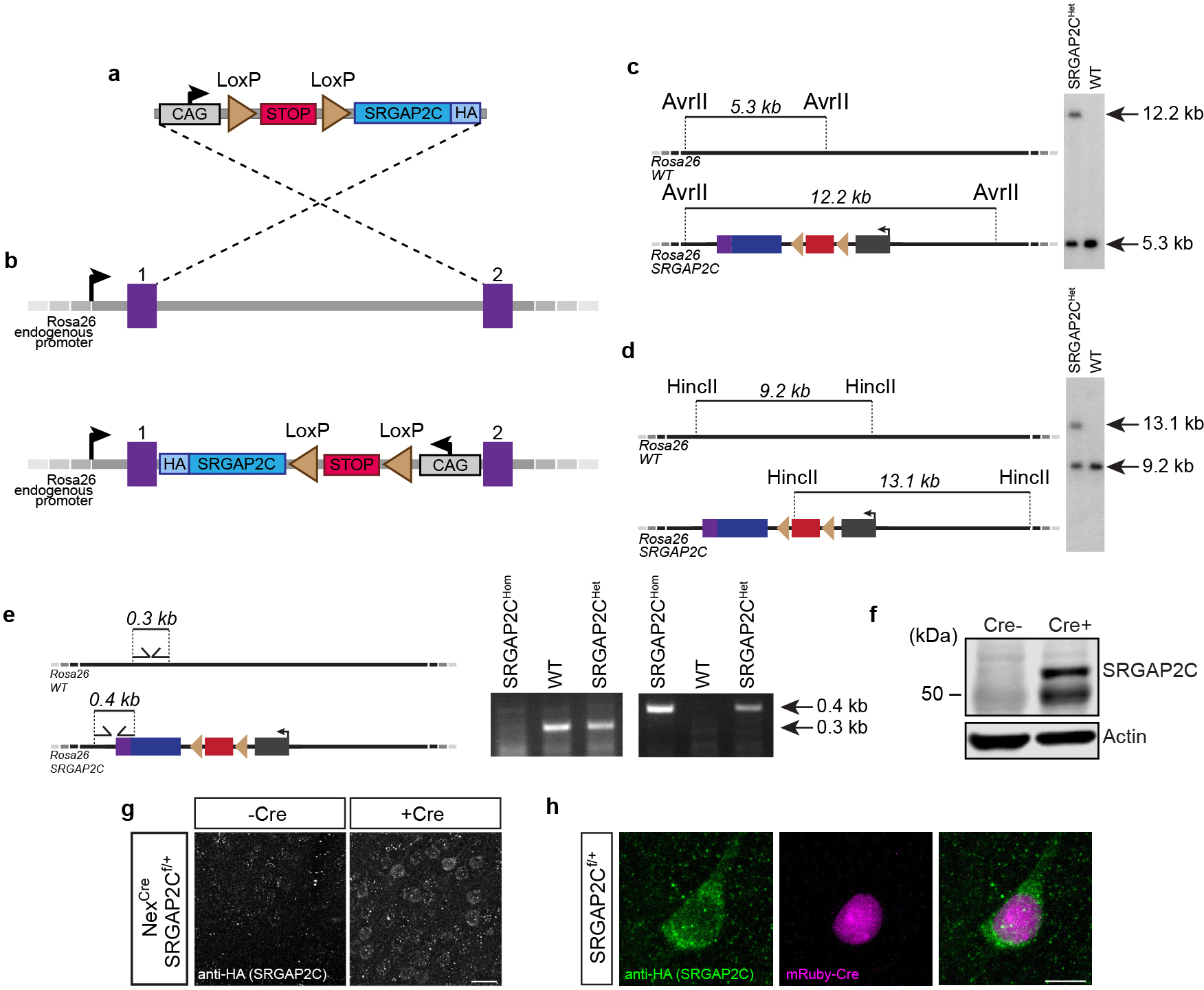
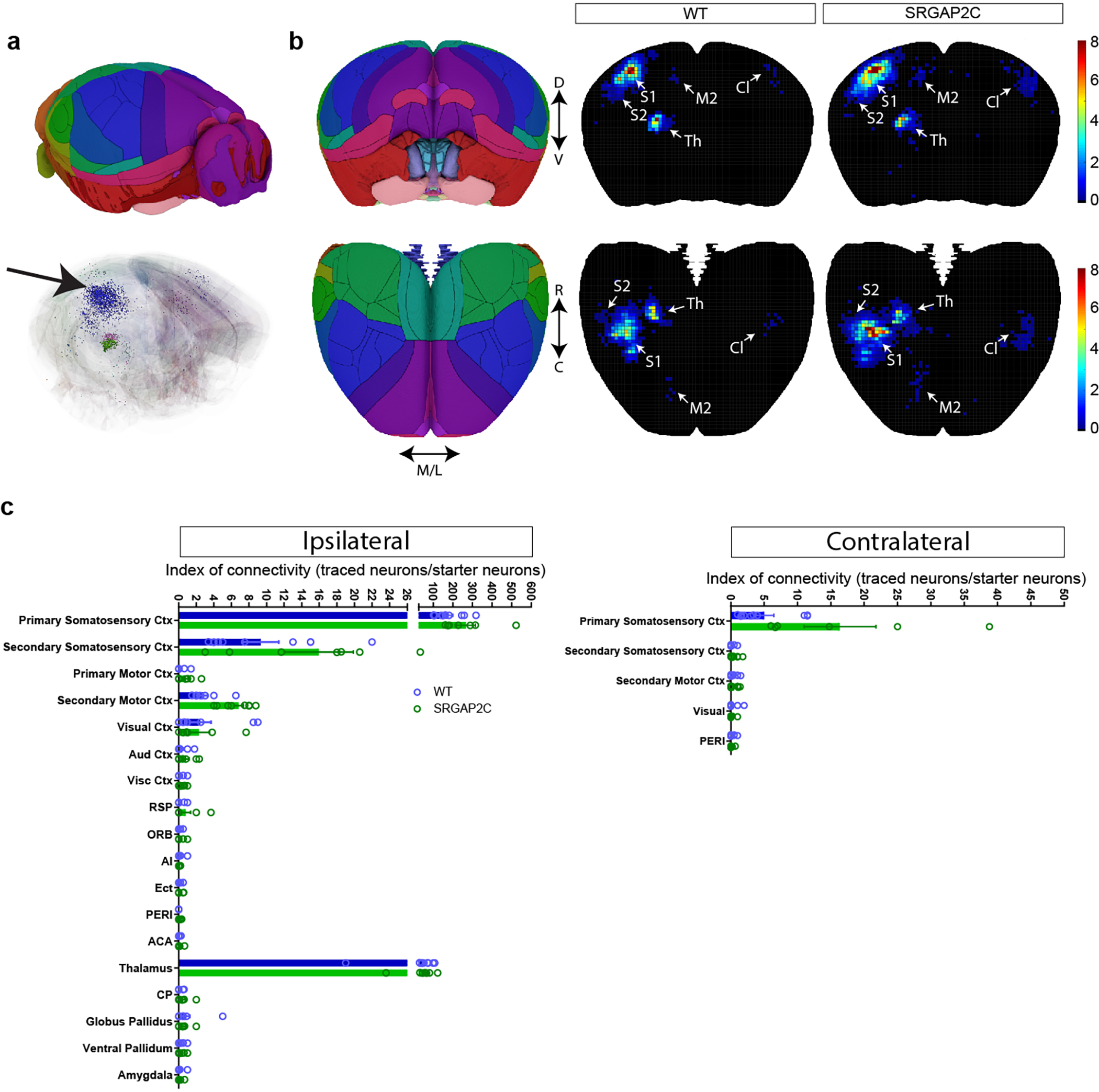
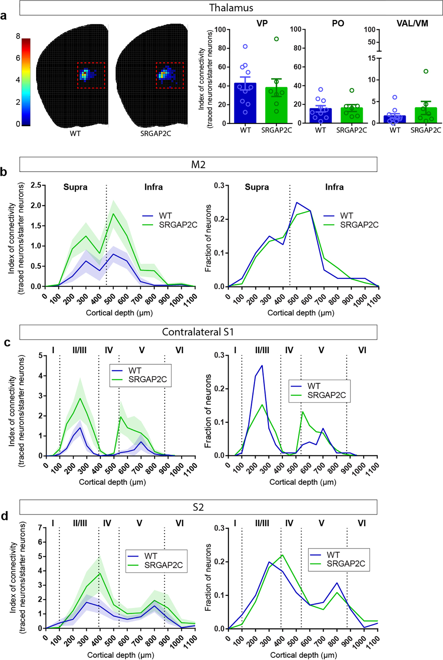
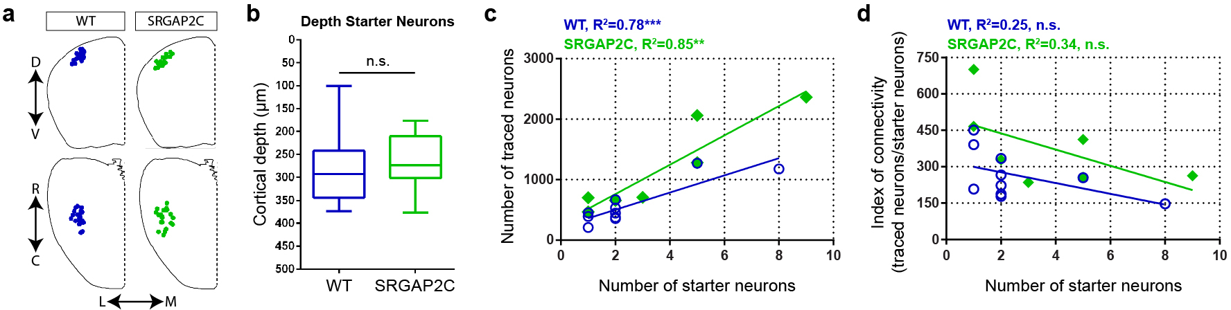
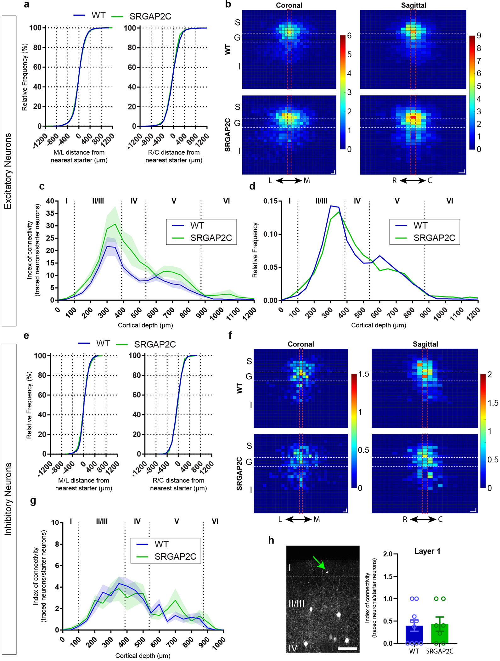
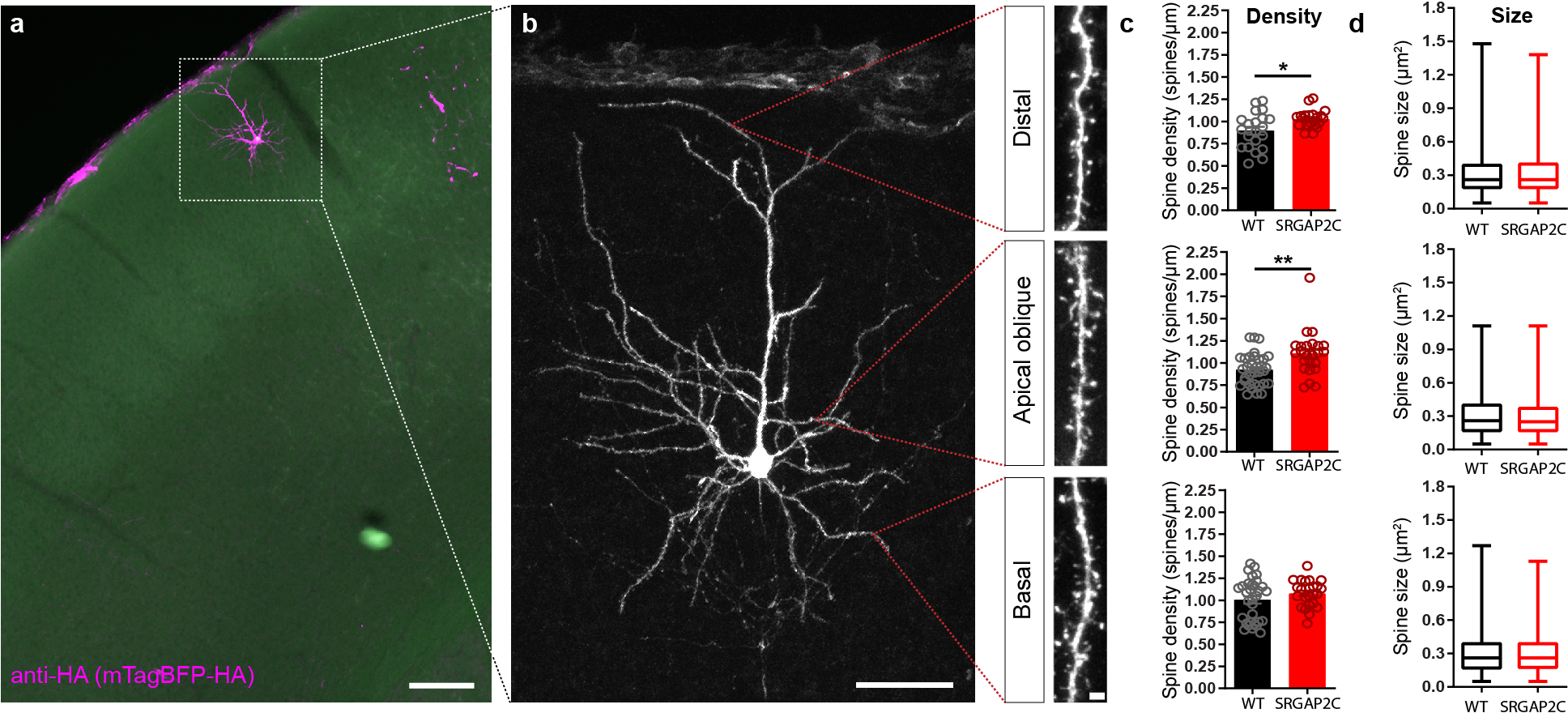
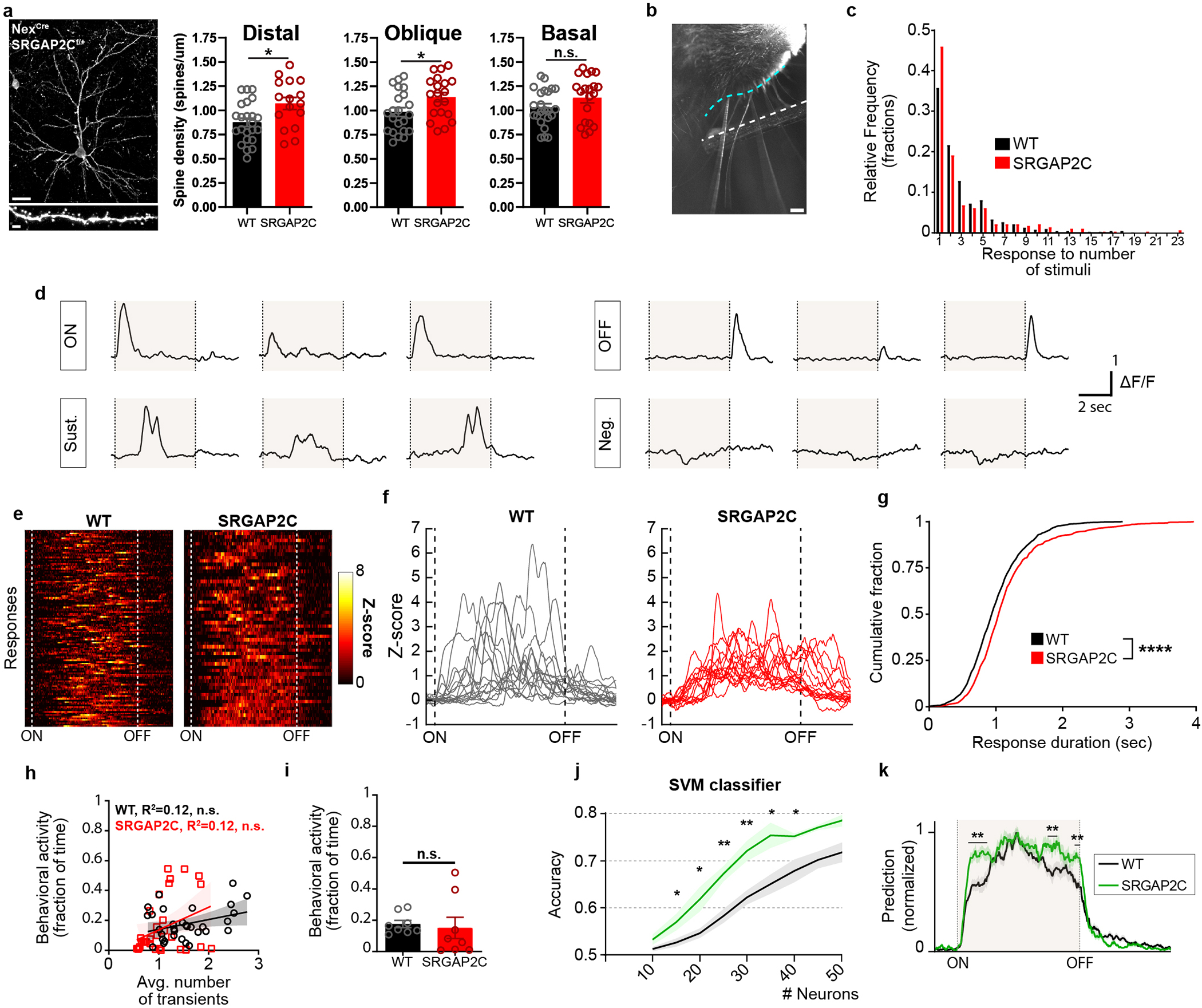
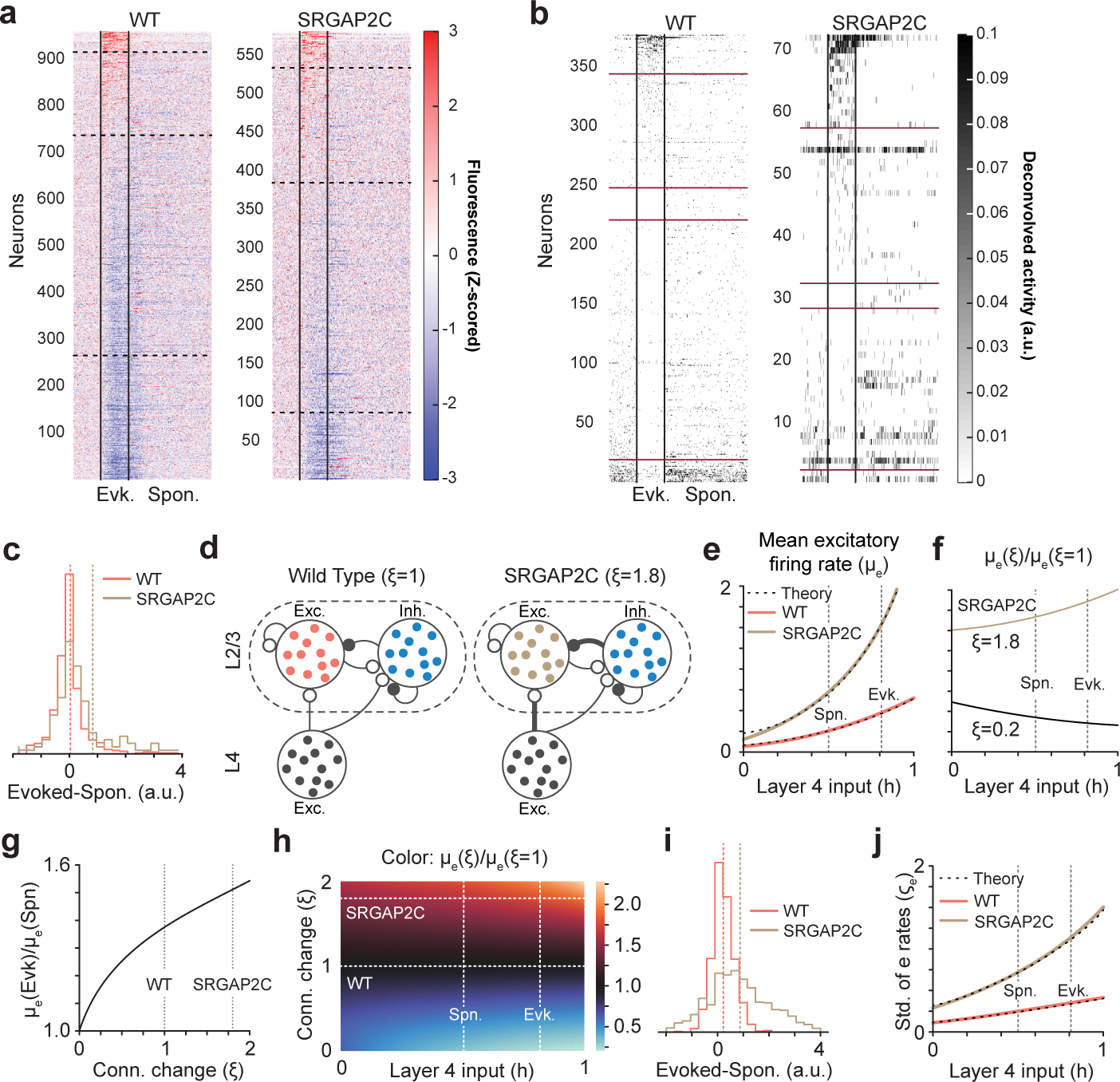
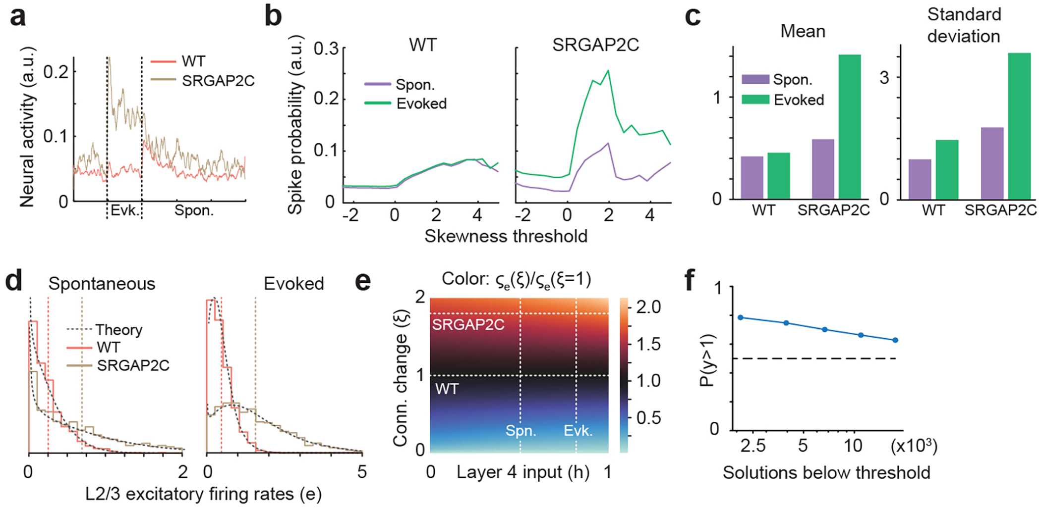
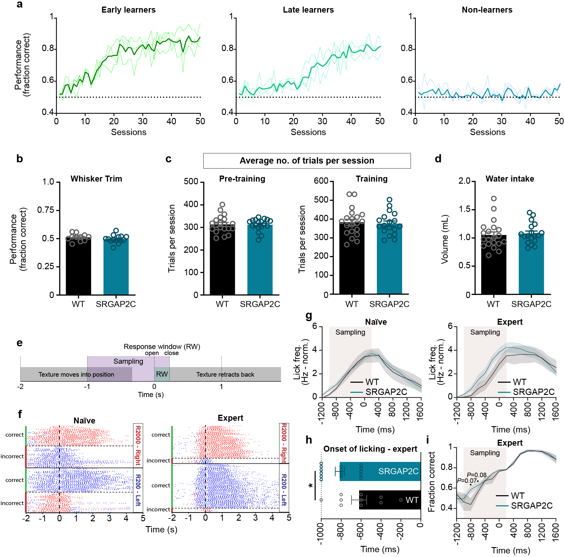
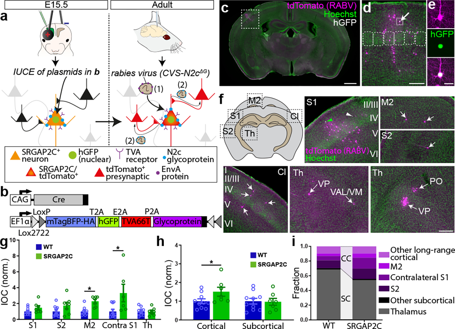
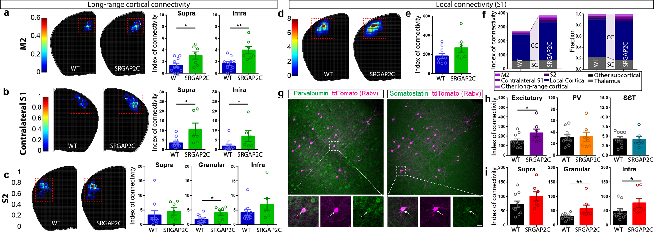
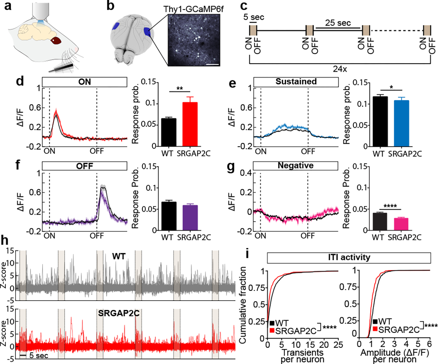
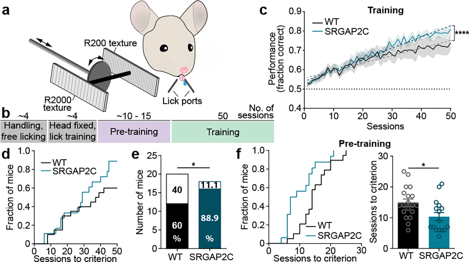
The cognitive abilities that characterize humans are thought to emerge from unique features of the cortical circuit architecture of the human brain, which include increased cortico-cortical connectivity. However, the evolutionary origin of these changes in connectivity and how they affected cortical circuit function and behaviour are currently unknown. The human-specific gene duplication SRGAP2C emerged in the ancestral genome of the Homo lineage before the major phase of increase in brain size^1,2. SRGAP2C expression in mice increases the density of excitatory and inhibitory synapses received by layer 2/3 pyramidal neurons (PNs)^3-5. Here we show that the increased number of excitatory synapses received by layer 2/3 PNs induced by SRGAP2C expression originates from a specific increase in local and long-range cortico-cortical connections. Mice humanized for SRGAP2C expression in all cortical PNs displayed a shift in the fraction of layer 2/3 PNs activated by sensory stimulation and an enhanced ability to learn a cortex-dependent sensory-discrimination task. Computational modelling revealed that the increased layer 4 to layer 2/3 connectivity induced by SRGAP2C expression explains some of the key changes in sensory coding properties. These results suggest that the emergence of SRGAP2C at the birth of the Homo lineage contributed to the evolution of specific structural and functional features of cortical circuits in the human cortex.

Extended Data Figure 1.. Generation of an inducible, humanized SRGAP2C transgenic mouse line.

(a-b) Design strategy for generating SRGAP2C conditional knock in mice. 3x HA tagged SRGAP2C was inserted into a Rosa26 targeting vector (a), which contains a CAG promoter, a floxed STOP-Neomycin cassette, and Rosa26 homology arms. Image not to scale. Using homologous recombination, the targeting vector was inserted between exon 1 and 2 of the Rosa26 locus (b). (c-d) Verification of SRGAP2C targeting in mouse embryonic stem cells using Southern blot analysis with probes that distinguish the targeted allele (12.2 kb in (c), 13.1 kb in (d)) from the wild-type allele (5.3 kb in (c), 9.2 kb in (d)). (e) Mice were genotyped by genomic PCR using the forward and reverse primers indicated that distinguish the WT Rosa26 allele or the SRGAP2C allele. (f) Western blot probed with anti-HA antibody of adult (P30) cortex isolated from SRGAP2C heterozygous conditional knock-in mice crossed with heterozygous Nex^Cre/+ mice (Cre+) or wild-type littermate (Cre-). The presence of Cre induces SRGAP2C-HA expression. Without Cre, no SRGAP2C was detected. Anti-Actin antibody was used as loading control. (g) Immunohistochemistry for HA on cortical brain sections from adult SRGAP2C heterozygous conditional knock-in mice crossed with heterozygous Nex^Cre/+ mice (Cre+) or wild-type littermate control (Cre-). Scale bar, 25 μm. (h) Same as g, on sections from SRGAP2C heterozygous conditional knock-in mice in which mRuby-Cre was sparsely expressed using in utero cortical electroporation. Scale bar, 10 μm.

Extended Data Figure 2.. Brain regions containing RABV traced neurons.

(a) Reference brain (top) based on Allen Reference Atlas. Digital reconstruction of RABV traced brain and registration onto reference brain. Black arrow indicates location of starter neurons in barrel field of S1. (b) Density plots showing distribution of traced neurons in WT and SRGAP2C mice. Colors in density plot indicate index of connectivity (IOC): number of traced neurons / number of starter neurons). (c) IOC for brain regions ipsilateral and contralateral to the injection site. RSP, retrosplenial area, ORB, Orbital cortex, Ai, Agranular Insular cortex, Ect, Ectorhinal cortex, PERI, Perirhinal cortex, ACA, Anterior Cingulate cortex, CP, Caudate-putamen. Bar graphs plotted as mean ± s.e.m. Open circles in bar graphs indicate individual mice (n = 10 for WT and n = 7 for SRGAP2C mice).

Extended Data Figure 3.. Distribution of RABV traced neurons.

(a) Index of connectivity (IOC, number of traced neurons / number of starter neurons) for traced neurons in the thalamus. No difference was observed between WT and SRGAP2C mice (two-sided Mann-Whitney test). Left: distribution of traced neurons in WT and SRGAP2C, colors indicate IOC. Right: IOC for Ventralanteriorlateral/medial (VAL/VM), Ventralposterior (VP), and Posterior (PO) thalamic subnuclei. Bar graphs plotted as mean ± s.e.m. Open circles in bar graphs indicate individual mice (n = 10 for WT and n = 7 for SRGAP2C mice). (b-d) Distribution of traced neurons as a function of their cortical depth. Left: IOC, right: fraction. Shaded area indicates s.e.m.

Extended Data Figure 4.. Connectivity changes are not caused by differences in cortical depth or number of starter neurons.

(a) Anatomical location of starter neurons. (b) Cortical depth of starter neurons measured as distance from pial surface is not different between WT and SRGAP2C mice, two-sided Mann-Whitney test. Data shown as box-and-whisker plots. Center line indicates median, box edges represent first and third quartiles, and whiskers represent minimum and maximum values (n = 26 starter neurons from 10 WT mice and n = 26 starter neurons from 7 SRGAP2C mice). (c) Correlation between number of RABV infected starter neurons and RABV traced neurons (Pearson’s correlation coefficient r = 0.88, P = 7 × 10⁻⁴ for WT, and r = 0.92, P = 3.2 × 10⁻³ for SRGAP2C). (d) No correlation was observed between IOC and number of RABV infected starter neurons per brain (Pearson’s correlation coefficient r = −0.5, P = 0.14 for WT, and r = −0.58, P = 0.17 for SRGAP2C).

Extended Data Figure 5.. Distribution of RABV traced neurons locally in S1.

(a) Distance between RABV traced excitatory neurons in S1 and their closest starter neuron along the medial/lateral (M/L) or rostral/caudal (R/C) plane. No difference was observed between WT and SRGAP2C mice (Kolmogorov-Smirnov test). Data shown as relative frequency distribution. (b) Density plots showing distribution of traced excitatory neurons relative to their closest starter neuron for coronal (left, L and M indicate lateral and medial orientation, respectively) and sagittal view (right, R and C indicate rostral and caudal orientation, respectively). Center bins aligned with relative position of starter neuron are indicated by red dashed lines. S, supragranular, G, granular, I, infragranular layers. For coronal, bin size = 50×50 μm. For sagittal, bin size = 50×100 μm. Colors in density plots indicate IOC. (c) Cortical layer distribution of RABV traced excitatory neurons in S1 shown as Index of connectivity (IOC, number of traced neurons / number of starter neurons). Shaded are indicates s.e.m. (d) Fraction of RABV traced neurons across cortical layers in S1. Dashed lines indicate borders between layers. Roman numbers identify cortical layers. (e) Same as (a), for inhibitory neurons. For analysis of interneurons, Parvalbumin-positive and Somatostatin-positive were grouped together. (f) Same as (b), for inhibitory neurons. (g) Same as in (c), for inhibitory neurons. Shaded are indicates s.e.m. (h) RABV traced neurons in layer 1. Left: Coronal section showing location of a layer 1 traced neuron (green arrow) in the barrel field of the primary sensory cortex (S1). Right: IOC for layer 1 traced neurons. No difference was observed between WT and SRGAP2C mice (Mann-Whitney test). Scale bar, 100 μm. Bar graphs plotted as mean ± s.e.m. Open circles in bar graphs indicate individual mice (n = 10 for WT and n = 7 for SRGAP2C mice).

Extended Data Figure 6.. SRGAP2C expression selectively increases synaptic density on apical dendrites.

(a) Coronal section stained for HA showing sparse labeling of a layer 2/3 cortical pyramidal neuron in the barrel field of the primary somatosensory cortex. Scale bar, 150 μm. (b) Higher magnification of neuron in (a). Red dotted lines indicate approximate location where spine density and size were quantified for distal, apical oblique, and basal dendritic compartments. Panels on right show high magnification images of dendritic segments on which spines can clearly be identified. Left panel scale bar, 50 μm. Right panel scale bar, 2 μm. (c) Spine density is increased for distal, and apical but not basal dendritic segments. (P = 1.92 × 10⁻² for distal, P = 1.5 × 10⁻³ for apical oblique, P = 0.3 for basal; distal: n = 21 segments for WT and SRGAP2C, apical oblique: n = 33 segments for WT and n = 24 segments for SRGAP2C, basal: n = 32 segments for WT and n = 24 segments for SRGAP2C). Bar graph plotted as mean ± s.e.m. *P < 0.05, **P < 0.01, two-sided Mann-Whitney test. (d) Spine size is not significantly changed in adult SRGAP2C expressing layer 2/3 cortical pyramidal neurons. Data shown as box-and-whisker plots. Center line indicates median, box edges represent first and third quartiles, and whiskers represent minimum and maximum values (distal: n = 1273 spines for WT and n = 1083 spines for SRGAP2C, apical oblique: n = 2401 spines for WT and n = 1650 spines for SRGAP2C, basal: n = 2286 spines for WT and n = 1448 spines for SRGAP2C).

Extended Data Figure 7.. Neuronal responses following whisker stimulation.

(a) Left: Coronal section stained for HA showing sparse labeling of a layer 2/3 cortical pyramidal neuron in the barrel field of the primary somatosensory cortex with high magnification (bottom) of dendritic segment in which spines can clearly be identified. Scale bar top, 25 μm. Scale bar bottom, 2 μm. Right: Spine density quantification in SRGAP2C heterozygous conditional knock-in mice crossed with heterozygous Nex^Cre/+ mice. Spine density is increased for distal and apical but not basal dendritic segments (P = 1.34 × 10⁻² for distal, P = 2.47 × 10⁻² for apical oblique, P = 0.117 for basal; distal: n = 23 segments for WT and n = 16 for SRGAP2C, apical oblique: n = 22 segments for WT and n = 20 segments for SRGAP2C, basal: n = 23 segments for WT and n = 20 segments for SRGAP2C). Bar graph plotted as mean ± s.e.m. *P < 0.05, two-sided Mann-Whitney test. (b) Top-down view of placement of stimulating rod (white dashed line, 2mm away from the whisker pad) next to right whisker pad (cyan dashed line). Scale bar, 1mm. (c) Frequency distribution of response fraction for neurons responding to either onset, sustained phase, or offset of the stimulus. (d) Singe-trial example responses. Shaded area indicates whisker stimulation. (e) Ten percent of single trial Sustained responses with longest sustained activity converted to Z-scores and sorted by duration of response. ON and OFF dashed lines indicate stimulus onset and offset, respectively (f) Bottom 15 responses shown in (e). (g) Cumulative probability distribution of Sustained response durations (time that Z-score was greater than 1). P < 1 × 10⁻⁴, Kolmogorov-Smirnov test. (h) Correlation between behavioral activity and average number of transients (n = 32 runs for 8 FOVs from 4 WT mice and n = 32 runs for 8 FOVs from 3 SRGAP2C mice). (i) Fraction of time during which behavioral activity was observed (n = 8 FOVs from 4 WT and n = 8 FOVs from 3 SRGAP2C mice). Bar graph plotted as mean ± s.e.m., two-sided Mann-Whitney test. (j) Support vector machine (SVM) accuracy in classifying presence or absence of whisker stimulus. Shaded area indicates s.e.m. (k) Normalized SVM prediction accuracy across time from stimulus ON to stimulus OFF for 25 neurons per field of view. Shaded area indicates stimulus time. Multiple t-test with multiple comparison correction using false-discovery rate Benjamini-Hochberg method (q < 0.05), *P < 0.05, **P < 0.01.

Extended Data Figure 8.. Computational modeling of increased layer 4 to layer 2/3 connectivity explains observed SRGAP2C neuronal response properties.

(a) Stimulus-triggered average fluorescence for all neurons recorded in WT and SRGAP2C mice. Fluorescence has been Z-scored and average activity during the 5 s prior to the stimuli have been subtracted. Horizontal dashed lines correspond to the separation between neurons that significantly increase (top) or decrease (bottom) their activity during evoked activity. Vertical solid lines correspond to stimulus onset and offset. Layer 2/3 PNs have been sorted according to the robustness of their signed response to the stimulus. (b) Stimulus-triggered average neural activity (after deconvolving fluorescence) for neurons with high signal-to-noise ratio. Horizontal red lines correspond to the separation between neurons that significantly increase (top) or decrease (bottom) their activity during evoked activity. Neurons between the middle horizontal red lines had an equal average response during spontaneous and evoked activity (typically 0). Neurons have been sorted according to the strength of their signed response to the stimulus. (c) The normalized distributions of firing rate differences between whisker stimulation and spontaneous activity. Dashed vertical lines indicate means of the distributions. (d) The model considers a population of excitatory neurons in layer 4 (gray) projecting to populations of inhibitory (blue) and excitatory (red, brown) neurons in cortical layer 2/3 of barrel cortex. The strength of the projections targeting layer 2/3 PNs and coming from layer 4 excitatory and layer 2/3 inhibitory neurons is assumed to be larger in SRGAP2C mice than WT mice by a factor ξ, as indicated. All neurons are modelled with a quadratic I/O transfer function. (e) The mean rate of simulated excitatory units (μ_e) in SRGAP2C mice (brown) are higher and increase at a higher rate than those in WT mice (red) as a function of the mean excitatory input h from layer 4. This is particularly true for the rates at the input levels we model as spontaneous and evoked activity (left and right gray vertical dashed lines, respectively). A mathematical approximation (black dashed lines; Supplementary Material) agrees to an excellent degree with the simulations. (f) The model ratio of mean excitatory rates between SRGAP2C mice (ξ = 1.8, top black curve) or mice with a hypothetical decrease in connection strength (ξ = 0.2, bottom black curve) and WT mice. (g) The model ratio between the mean excitatory rate during evoked vs. spontaneous activity monotonically increases with the change in connectivity relative to WT mice. (h) The model ratio of mean excitatory rates between mice with an arbitrary change in connection strength and WT mice. (i) The normalized distributions of firing rate differences between evoked and spontaneous mean input in the model. As in the experimental data (panel c), both model SRGAP2C and model WT mice contain subgroups of neurons that increase and subgroups that decrease their activity in going from spontaneous to evoked stimulation; and the fraction of neurons increasing their activity is higher in SRGAP2C mice than WT mice. (j) As for the mean rates (panel e), the variances of excitatory units in model SRGAP2C mice (brown) are higher, and increase at a higher rate as a function of the mean excitatory input from layer 4, than those in model WT mice (red).

Extended Data Figure 9.. Modeling of layer 2/3 PN response properties in WT and SRGAP2C mice.

(a) Population stimulus-triggered-average neural activity obtained by averaging over all neurons in Extended Data Figure 8b. Vertical dashed lines correspond to stimulus onset and offset. (b) Average neural activity computed during the 5 s before the stimulus (Spon.) or during the 5 s of stimulation (evoked; stimulus is applied at time 0) across all selected neurons and trials as a function of the skewness threshold used to select neurons. The threshold in (a) is 1.5. (c) Mean and standard deviation of the deconvolved traces in Extended Data Figure 8b during both stimulus conditions. (d) The normalized distributions of simulated excitatory rates in both SRGAP2C (brown) and WT (red) mice and during spontaneous and evoked mean input illustrate the increase in the mean and variance discussed in the main text. The shapes of the distributions agree with their mathematical approximations (dashed black line) discussed in Supplementary Material. (e) The ratio of the standard deviation of excitatory rates between mice with an arbitrary change in connection strength and WT mice. This demonstrates that the effects are robust to the specific choice of parameters. (f) Probability of solutions with y>1 as a function of the number of solutions with a fit error of the firing rates of the wild type mouse below a certain threshold, where y = [mu(2c,evoked)/mu(2c,spont)]/[mu(wt,evoked)/mu(wt,spont)] and mu corresponds to the mean firing rate of the excitatory population.

Extended Data Figure 10.. Whisker-based texture discrimination task.

(a) Example learning curves (lighter shades) of three individual mice. Mean learning curve is shown in darker shade (b) Performance (fraction correct) after whiskers facing texture were trimmed dropped to chance level, showing that mice needed their whiskers to perform this task (n = 11 for WT and n = 14 for SRGAP2C mice). (c) Average number of trials per session for pre-training and training phase (n = 20 for WT and n = 18 for SRGAP2C mice). (d) Mean water intake per session (n = 20 for WT and n = 18 for SRGAP2C mice). Bar graphs plotted as s.e.m. (e) Schema showing structure of single trial. Textures rotate and move into position 2 s before opening of the response window (RW). Approximately 1 s before RW opening the texture is within reach of the whiskers, allowing mice to sample the texture while it moves further into position. Upon opening of the RW, correct lick responses lead to a water reward, while incorrect lick responses cause to a time-out. Following RW closure the texture retracts back out of reach of the whiskers. (f) Example raster plot of an individual mouse showing the distribution of individual licks (red dot for right licks, blue dot for left licks) relative to opening of the response window before (naïve) and after (expert) learning of the task. Correct licks are either right licks (red) for the R2000 texture, or left licks (blue) for the R200 texture. (g) Lick frequency plot for naïve and expert mice. Lick frequency was normalized for each individual mouse to the mean lick frequency before the sampling window. Shaded area around curves indicates s.e.m. (h) Average timing of licking onset in expert mice relative to opening of the response window (P = 4.91 × 10⁻²; n = 10 for WT and n = 15 for SRGAP2C mice). Bar graph plotted as mean ± s.e.m. *P < 0.05, two-sided Mann-Whitney test. (i) Fraction of licks from expert mice that are correct relative to opening of the response window. Shaded area around curves indicates s.e.m., two-sided Mann-Whitney test.

Figure. 1.. Sparse monosynaptic tracing in layer 2/3 PNs humanized for SRGAP2C expression.

(a) The BHTG construct (see b), together with Cre recombinase, is targeted to layer 2/3 cortical PNs in S1 by in utero electroporation (IUCE) at E15.5. Stereotactic injection of RABV in adult mice leads to infection of starter neurons (1), after which it spreads to presynaptically connected neurons (2). (b) BHTG and Cre constructs. (c) Coronal section stained for Hoechst (green) showing location of a starter neuron (dashed white box) in the barrel field of the primary sensory cortex (S1). Scale bar, 1 mm. (d) Higher magnification of dashed white box area in (c). Starter neuron indicated by white arrow. Rounded boxes indicate barrels in layer 4. Scale bar, 200 μm. (e) High magnification of starter neuron. Scale bar, 25 μm. (f) Anatomical location of RABV traced neurons. Green arrowhead in S1 indicates RABV infected starter neuron. White arrowheads mark non-infected, electroporated neurons. White arrows mark RABV traced neurons. Roman numbers identify cortical layers. Scale bar, 250 μm. (g) Index of connectivity (IOC) for brain regions in (f), relative to control. P = 2.54 × 10⁻² for M2 and P = 1.56 × 10⁻² for contralateral S1. *P < 0.05, Kruskal-Wallis test. (h) IOC relative to control for cortical and subcortical inputs. P = 3.33 × 10⁻² for cortical and P = 0.98 for subcortical. Bar graphs plotted as mean ± s.e.m. Open circles in bar graphs indicate individual mice (n = 10 for WT and n = 7 for SRGAP2C mice), *P < 0.05, two-sided Mann-Whitney test. (i) Fraction of inputs for all RABV traced long-range inputs.

Figure. 2.. SRGAP2C expression increases cortical inputs onto layer 2/3 PNs.

(a-c) Index of connectivity (IOC) for M2, contralateral S1, and S2. Left: distribution of traced neurons. Colors in density plot indicate IOC. Right: IOC. M2: P = 2.99 × 10⁻² for supragranular and P = 4.1 × 10⁻³ for infragranular; Contralateral S1: P = 1.77 × 10⁻² for supragranular and P = 1.39 × 10⁻² for infragranular; S2: P = 2.63 × 10⁻² for granular; two-sided Mann-Whitney test. (d) Distribution of locally traced neurons in S1, colors indicate IOC. (e) IOC for S1. P = 0.109, two-sided Mann-Whitney test. (f) IOC (left) and fraction (right) for all RABV traced inputs, including local cortical inputs originating in S1. (g) Double immunohistochemistry of the same RABV traced brain section for PV (top) and SST (bottom). Bottom panels represent higher magnification of area indicated by dashed boxes. Scale bar large panel, 200 μm. Scale bar small panel, 20 μm. (h) IOC for excitatory, PV-positive, and SST-positive RABV traced neurons in S1. P = 3.3 × 10⁻² for excitatory, two-sided Mann-Whitney test. (i) IOC for excitatory neurons in supragranular, granular, and infragranular layers of S1. P = 6.8 × 10⁻³ and P = 4.31 × 10⁻² for excitatory neurons in the granular and infragranular layer, respectively. Bar graph plotted as mean ± s.e.m. Open circles in bar graphs indicate individual mice (n = 10 for WT and n = 7 for SRGAP2C mice), *P < 0.05, **P < 0.01, two-sided Mann-Whitney test.

Figure. 3.. SRGAP2C increases probability and selectivity of neuronal responses to sensory stimulation.

(a-c) Schema of experimental approach. (d-g) Left panels: average calcium traces (ΔF/F) for indicated response types. Shaded area indicates s.e.m. Right panels: response probability expressed as fraction of stimuli leading to a response. P = 6.4 × 10⁻³ for ON, P = 4.31 × 10⁻² for Sustained, and P = 3.21 × 10⁻¹ for OFF. Bar graph plotted as mean ± s.e.m. *P < 0.05, **P < 0.01, ****P < 0.0001, two-sided Mann-Whitney test. (h) 150 randomly chosen Z-scored example traces showing activity during six consecutive stimuli (shaded) and corresponding ITIs. (i) Cumulative probability distribution of Ca²⁺ transient number and amplitude during intertrial interval (ITI). ****P < 0.0001, Kolmogorov-Smirnov test (n = 580 neurons for WT and n = 277 neurons for SRGAP2C).

Figure. 4.. Humanized SRGAP2C mice display increased ability to learn a texture discrimination task.

(a-b) Schematic of whisker-based texture discrimination task. Distance between laser cut grooves for R200 and R2000 textures is 200 and 2000 μm, respectively. Scale bar, 100 μm. (c) Behavioral performance shown as fraction of correct trials over sessions of training (1 session / day). Shaded area indicates s.e.m. Linear regression indicated by dashed lines. Dotted horizontal line indicates chance level performance (50% correct). Linear regression, slope WT = 0.0039, slope SRGAP2C = 0.0057. ****P < 0.0001, linear regression F-test. (d) Cumulative histogram for number of sessions to learning criterion (75% correct). (e) Number of learners (mice that reached 75% correct responses) and non-learners (mice that never reached 75% correct responses). Numbers in bar graphs indicate percentage of total number of mice tested. P = 0.043, Chi-Square test. (f) Left: cumulative histogram for number of sessions to learning criterion during pre-training (75% correct responses). Right: number of sessions to reach criterion. P=0.0135, two-sided Mann-Whitney test. Bar graphs plotted as mean ± s.e.m. Open circles in bar graphs indicate individual mice (n = 19 for WT and n = 16 for SRGAP2C mice), *P < 0.05.

References

1. Dennis MY et al. The evolution and population diversity of human-specific segmental duplications. Nat. Ecol. Evol. 1, 0069 (2017). - PMC - PubMed
1. Ponce de León MS et al. The primitive brain of early Homo. Science 372, 165–171 (2021). - PubMed
1. Charrier C et al. Inhibition of SRGAP2 function by its human-specific paralogs induces neoteny during spine maturation. Cell 149, 923–35 (2012). - PMC - PubMed
1. Fossati M et al. SRGAP2 and Its Human-Specific Paralog Co-Regulate the Development of Excitatory and Inhibitory Synapses. Neuron 91, 356–369 (2016). - PMC - PubMed
1. Schmidt ERE, Kupferman JV, Stackmann M & Polleux F The human-specific paralogs SRGAP2B and SRGAP2C differentially modulate SRGAP2A-dependent synaptic development. Sci. Rep. 9, 18692 (2019). - PMC - PubMed
Publication types