Central nervous system physiology

Abstract

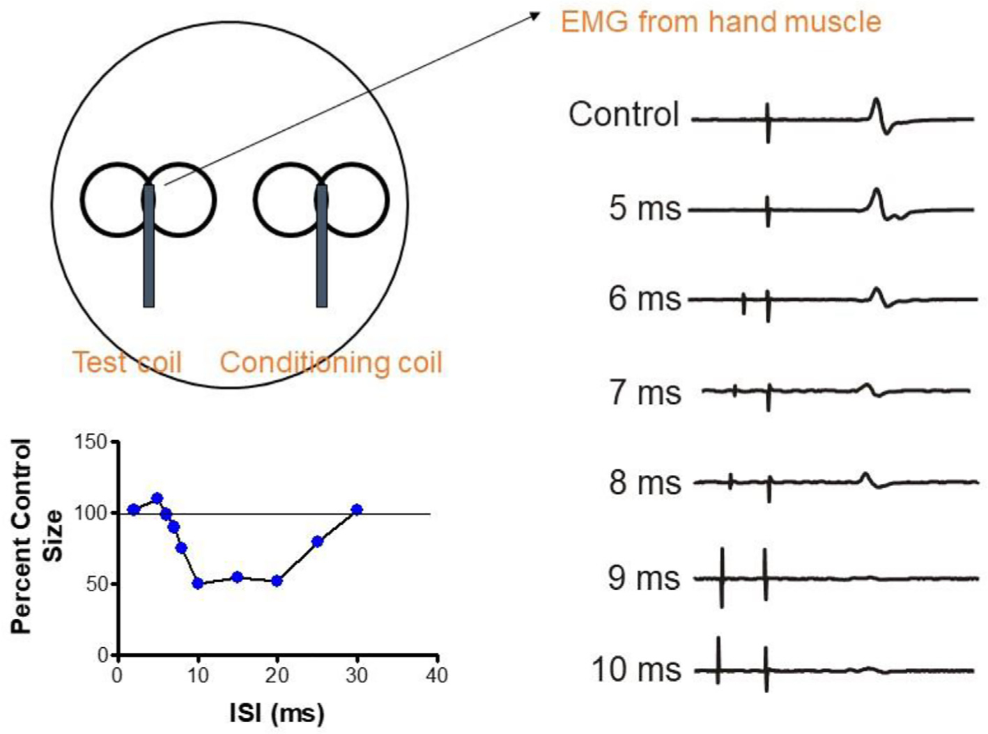
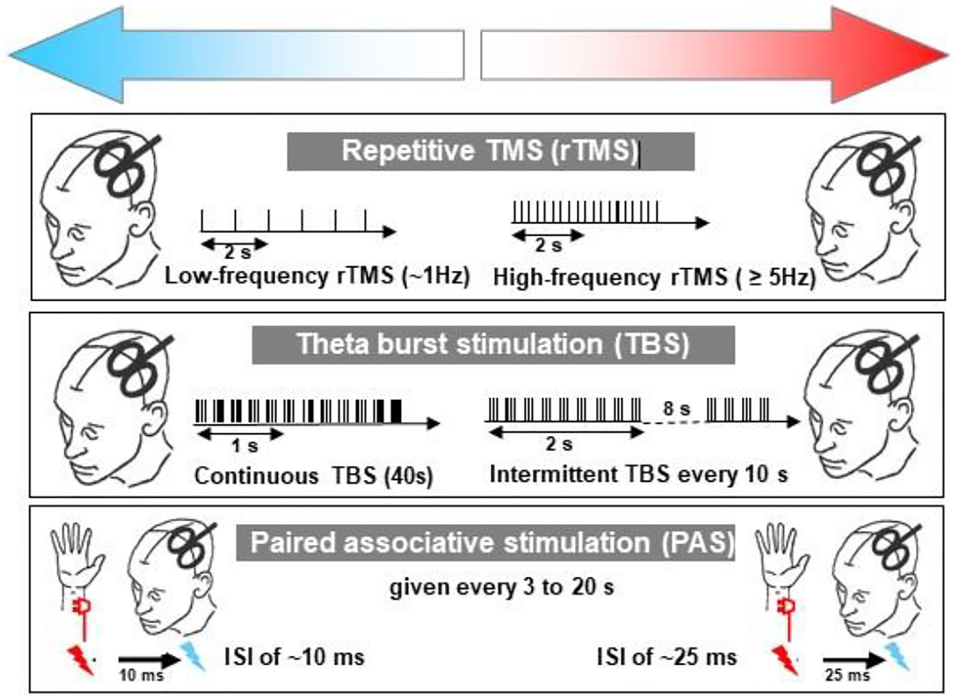
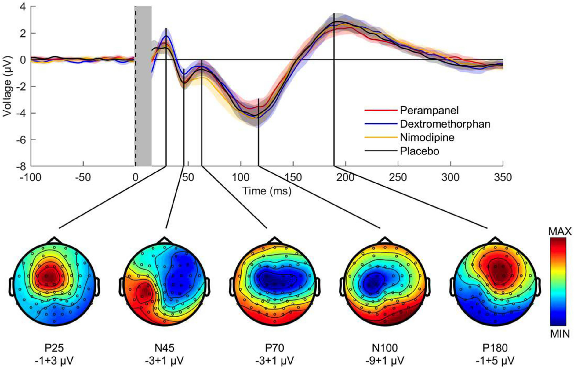
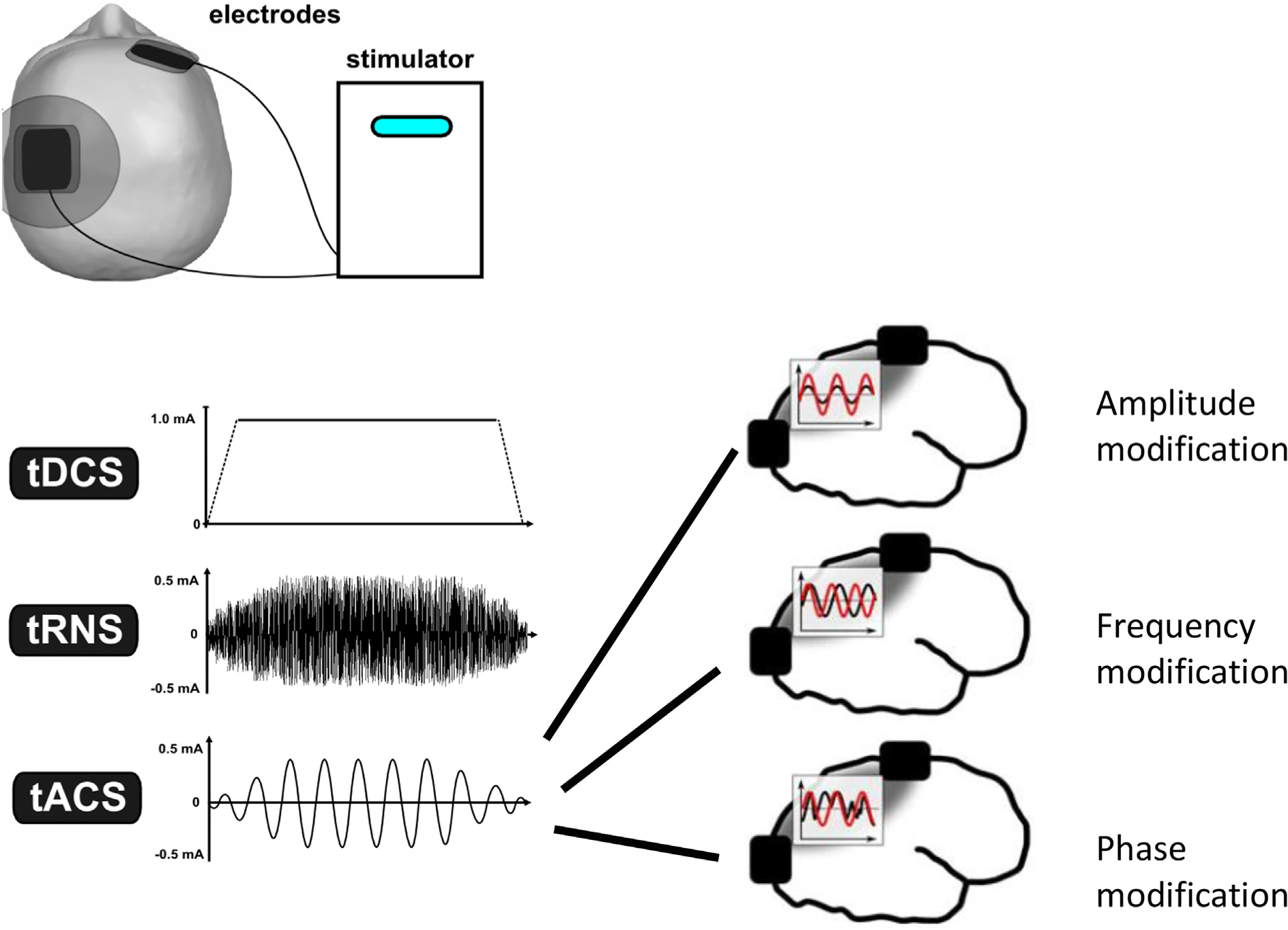
This is the second chapter of the series on the use of clinical neurophysiology for the study of movement disorders. It focusses on methods that can be used to probe neural circuits in brain and spinal cord. These include use of spinal and supraspinal reflexes to probe the integrity of transmission in specific pathways; transcranial methods of brain stimulation such as transcranial magnetic stimulation and transcranial direct current stimulation, which activate or modulate (respectively) the activity of populations of central neurones; EEG methods, both in conjunction with brain stimulation or with behavioural measures that record the activity of populations of central neurones; and pure behavioural measures that allow us to build conceptual models of motor control. The methods are discussed mainly in relation to work on healthy individuals. Later chapters will focus specifically on changes caused by pathology.

Keywords: Bereitschaftspotential; Computational motor control; Evoked potential; Reaction time; Transcranial direct current stimulation; Transcranial magnetic stimulation.

Fig. 1.

Some spinal circuits that can be tested reliably in human subjects. Group Ia circuits in red; group II circuits in blue; descending controls in green. IN: interneuron. MN: motoneuron. PAD INs: interneurones that produce primary afferent depolarisation and are, thereby, responsible for presynaptic inhibition. HD: homosynaptic depression (=post-activation depression of transmitter release at the synapse). NA: brainstem noradrenergic pathway (suppressing group II reflex excitation). RC: Renshaw cell. From (Pierrot-Deseilligny and Burke, 2012) with permission.

Fig. 2.

H reflexes of abductor pollicis brevis during a voluntary contraction and F waves of the thenar muscles in the same subject. A, H reflex recorded using unrectified electromyography (EMG) (4 averages, each of 32 sweeps), as used to calculate H-reflex latencies. B, H reflex recorded using rectified EMG (3 averages, each of 32 sweeps). C, F waves of abductor pollicis brevis (APB) (3 averages, each of 32 sweeps). Note the small M wave in A and B, and the maximal M wave in C. The F wave latency is slightly shorter than the H reflex latency (on average the latency of the H reflex of APB = ~1.1 × latency of fastest F wave. From (Espiritu et al., 2003), with permission.

Fig. 3.

Inability of the H reflex to detect reflex actions mediated through interneurons. Panel (a) shows the circuitry proposed to explain the data in panel (b). Stimulation of the superficial (cutaneous) branch of the radial nerve at the wrist inhibits propriospinal neurons located at the C3-C4 level, thus reducing the component of the corticospinal volley transmitted to the motoneuron pool of extensor carpi radialis (ECR). Panel (b) shows that cutaneous afferents in the radial nerve supressed the background electromyography (EMG) of a steady voluntary contraction of ECR (filled circles) and the motor evoked potential (MEP) of the contracting ECR (filled triangles), but did not significantly suppress the H reflex of contracting ECR (open circles). The inhibition was therefore not at the motoneuron, and must have occurred at an interneuron, involving “disfacilitation”, rather than direct inhibition. The central delay, i.e., the extra interval spent within spinal cord circuitry, was 4 ms, which is too short for a pathway outside the spinal cord. This is consistent with transmission through propriospinal neurons located a few segments above the motoneuron pool. From (Pierrot-Deseilligny and Burke, 2012) with permission.

Fig. 4.

Reflexly activated motoneurons cannot produce F waves. In human subjects, the supramaximal stimulus necessary for F wave studies will produce an intense afferent volley. If motoneurons are activated by this afferent input, the reflex discharge will collide with the antidromic volley in motor axons, thus preventing the antidromic invasion of those motoneurons (the two motoneurons on the left). As a result, F waves will occur only for higher-threshold motoneurons that have a smaller compound excitatory post-synaptic potential (EPSP) and do not discharge reflexly in response to the afferent volley. From (Mills, 2017) with permission.

Fig. 5.

Simple schematic drawing of the circuits leading to blink and startle reflexes. Inputs from many sources impinge on the trigeminal complex (V) and the various structures of the reticular formation (RF). Output projections from V lead to R1 and R2 responses of the blink reflex. The difference in thickness of the arrows pointing to R1 and R2 responses mark their different behavior to conditioning experiments (see text). The R2 response can also be generated by inputs from other sources. Output projections from RF go to motoneurons of the facial and other brainstem nuclei, as well as to spinal cord alpha motoneurons. Additionally, inputs are processed in the prepulse circuit (pP), causing inhibition of the R2 and the startle reflex responses (broken line arrows).

Fig. 6.

Responses of the orbicularis oculi muscle, as part of blink reflexes, elicited by 1) electrical stimuli to the supraorbital nerve (V1), which generates the R1 and R2 responses, 2) an unexpected tap to the mandible with a sweep-triggering hammer (TAP), which generates an R2 response, 3) an electrical stimulus to the median nerve (MN), which generates the so-called hand blink reflex (HBR), and 4) a loud acoustic stimulus (AUD), which generates the so-called auditory blink reflex (ABR).

Fig. 7.

Startle reaction to an unexpected loud auditory stimulus (110 dB). In A, responses were recorded while the subject was at rest. In B, responses were recorded when the same subject was ready to perform a fast wrist extension movement at perception of the auditory signal. Note the enhancement of the responses recorded from the Orbicularis Oculi (OOc) and the sternocleidomastoid (SCM), and the burst of activity recorded from the wrist extensor muscles (WE), leading to the wrist extension movement (MOV).

Fig. 8.

Representative examples of prepulse inhibition of the blink reflex to a supraorbital nerve stimulus (A) and of the startle reaction to a loud auditory stimulus. The same stimuli are presented in the traces at the top and at the bottom, except that, at the bottom, a prepulse stimulus (pP), a low intensity electrical stimulus to the second digit of the right hand (incapable of eliciting any reflex response by itself), precedes the reflex-eliciting stimuli (S) by 100 ms. Note the suppression of the R2 and R2c responses of the blink reflex, with the enhancement of the R1, and the suppression of all responses to the startling stimulus.

Fig. 9.

Descending volleys evoked by electrical and magnetic stimulation and by paired pulse magnetic stimulation. Each trace is the average of the responses to 10–25 cortical stimuli, recording shown in the three columns have been obtained in three different subjects. Electrical anodal stimulation at threshold intensity evokes the earliest volley that is termed D-wave. Low intensity magnetic stimulation with a posterior-anterior (PA) induced current in the brain evokes a single descending wave with a latency about 1 ms longer than the D-wave evoked by electrical stimulation that is termed I1 wave. At intermediate intensity later I-waves are evoked and at high intensity, an earlier small wave with the same latency of the D wave evoked by electrical anodal stimulation appears. Magnetic stimulation with a latero-medial (LM) induced current in the brain preferentially evokes D-wave activity. With biphasic magnetic stimulation the earliest volley has a latency of about 0.4 millisecond longer than the D wave evoked by LM magnetic stimulation. Because of its longer latency, it is suggested that the D wave evoked by biphasic stimulation is initiated closer to the cell body of the PTNs than the conventional D wave evoked by LM magnetic stimulation and anodal stimulation and it is termed “proximal D wave”). On the right, epidural volleys evoked by test magnetic stimulus alone (solid trace) and by test magnetic stimulus preceded by a subthreshold conditioning stimulus at 3 milliseconds interstimulus interval (dotted trace). The test stimulus evokes multiple descending waves. There is a clear suppression of the late corticospinal volley when the test magnetic stimulus is preceded by the subthreshold conditioning stimulus. From (Di Lazzaro and Rothwell, 2014) with permission.

Fig. 10.

Interhemispheric inhibition between the motor cortices. A suprathreshold TMS pulse (test pulse) is applied to the left hemisphere to evoke a motor evoked potential (MEP) (control trace in right panel). If a conditioning TMS pulse is applied 5–10 ms beforehand, it suppresses the amplitude of the evoked MEP, starting at an interval of 6 ms. The panel in the bottom left shows the time course of inhibition, where the amplitude of the control MEP is set to 100%. The duration and depth of inhibition depend on the intensity of the conditioning stimulus (not shown).

Fig. 11.

Three methods of inducing long-term potentiation/depression (LTP/LTD) -like effects in human motor cortex that have been used to explore cortical plasticity in dystonia. In all cases, motor excitability is assessed by measuring the electromyography (EMG) response to a standard single TMS pulse before and at various times after the plasticity inducing protocol. Protocols on the left of the panel all decrease (upper blue arrow) cortical excitability whereas those on the right all increase excitability (upper red arrow). The protocol in the upper three panels involves repeated TMS pulses. In the top panel TMS is applied at a regular intervals until 1000–1500 total stimuli have been given. If the pulses are given at a frequency of 5 Hz or more they facilitate whereas a frequency of 1 Hz depresses excitability for 30–60 min. In the second panel, the TMS pulses are applied in high frequency bursts of 3 pulses at 50 Hz, repeated five times per second. These are “theta burst” paradigms, so called because the theta rhythm in EEG has a frequency of 5 Hz. Bursts that are applied intermittently (2 s on, 8 s off, repeated 20 times; 600 total TMS pulses) cause facilitation whereas continuous theta bursts for 40 s (a total of 600 pulses) lead to suppression. The third panel shows a method based on descriptions of Hebbian plasticity. Each TMS pulse is applied in close temporal relation to an electrical stimulus of the median nerve at the wrist. If the stimuli are timed with an interval of 25 ms then the afferent input from the median nerve stimulus reaches motor cortex just before the TMS is given. In this condition, repeated pairings (usually 90–100 given every 2–3 s) lead to facilitation, whereas if the interval between pulses is 10 ms there is suppression of excitability. From (Quartarone et al., 2006) with permission.

Fig. 12.

Group average of pre-drug TMS-evoked EEG potentials (TEPs) after stimulation of left motor cortex. Top panel: pre-drug TEPs averaged across all subjects (n = 16) and EEG electrodes for perampanel (red curve), dextromethorphan (blue curve), nimodipine (yellow curve) and placebo (black curve). Shades represent ± 1 SEM. The vertical gray bar represents the time window affected by the TMS artefact that was removed and interpolated. Note excellent reproducibility of TEPs at group level across baseline sessions. Bottom panel: pre-drug TEP topographies averaged across subjects (n = 16) and drug conditions. Each topography was obtained by averaging the signal in the respective time window of interest (P25: 16–34 ms, N45: 38–55 ms, P70: 56–82 ms, N100: 89–133 ms, P180: 173–262 ms). Data are voltages at sensor level (ranges indicated underneath the plots), while colors are normalized to maximum/minimum voltage (from (Belardinelli et al., 2021), with permission).

Fig. 13.

During electrical stimulation current flows between two electrodes. During tDCS, direct (i.e. steady) current is applied; tRNS uses a mixture of oscillating currents with a frequency range between 0.1 Hz and 640 Hz; and during tACS oscillating electric fields of a single frequency are applied. The panels on the right of the figure show how the parameters of tACS can be varied: amplitude and frequency at a single pair of electrodes can be adjusted, whereas if tACS is applied through two (or more) electrode pairs, the phase of the oscillations between the sites can also be adjusted. tACS: transcranial alternating current stimulation; tDCS: transcranial direct current stimulation; tRNS: transcranial random noise stimulation.

Fig. 14.

Schematic representation of information processing stages occurring in various reaction time (RT) tasks.

Fig. 15.

Schematic representation of different measures of reaction time (RT) in a single theoretical choice RT trial requiring a finger-lift off a button. Time zero indicates onset of the informative go-stimulus, with each theoretical signal shown with respect to its own baseline (offset vertically for visibility). Signals include electromyography (EMG) from the responding finger (blue), lateralized readiness potential (LRP) from electroencephalography (EEG) (purple), motor evoked potential (MEP) amplitude from motor cortex contralateral to responding limb (brown), displacement of the finger (black) - along with differentiated velocity and acceleration (dark grey, light grey), and force applied (red) with button state (green). Arrows on each trace (with corresponding numbers below the time scale) indicate the theoretical threshold-based time-detection of a change in that signal. For example premotor RT in EMG is shown with blue arrow and number 3. Durations of each information processing stage (black boxes) are not to scale, but note that onset of LRP roughly corresponds to completion of response selection (*Note that this theoretical representation of a single trial timeline is based on composite data from (Brenner and Smeets, 2019; Leocani et al., 2000; Leuthold et al., 2004; Maslovat et al., 2020)).

Fig. 16.

Slow shifts of the Bereitschaftspotential (BP) preceding volitional, rapid fixations of the right index finger (t = 0 s, vertical line). Recording positions are left precentral (L prec, C3), right precentral (R prec, R4), mid-parietal (Pz). Unipolar recordings with linked ears as reference. The difference between BP in C3 and C4 is displayed in the lowest graph (L/R prec). Superimposed are the results of eight experiments as obtained in the same subject on different days. Note that BP has two components, the early one (BP1) lasting from app. −1.2 to −0.5 s; the late component (BP2) from −0.5 to shortly before 0 s. (From (Deecke and Kornhuber, 2002) and adapted with permission.)

Fig. 17.

Derivation of the Lateralized Readiness Potential (LRP) with the double subtraction method on the basis of Event Related Potential (ERP) waveforms elicited at electrodes C3′ (left hemisphere) and C4′ (right hemisphere). Top: Grand-averaged ERP waveforms from ten participants elicited at C3′ (solid lines) and C4′ (dashed lines) in response to stimuli requiring a left-hand response (left side) or a right-hand response (right side). Bottom left: Difference waveforms resulting from subtracting the ERPs obtained at C4′ from the ERPs obtained at C3′ separately for left-hand responses (solid line) and right-hand responses (dashed line). Bottom right: LRP waveform resulting from subtracting C3′-C4′ difference waveform for right-hand responses from the C3′-C4′ difference waveform from left-hand responses. A downward-going (positive) deflection indicates an activation of the correct response, and upward-going (negative) deflection indicates an activation of the incorrect response. (From (Jahanshahi and Hallett, 2002a) adapted and reprinted with permission.)

Fig. 18.

A. Evoked potentials (EPs) recorded over the frontal cortex in response to clicks; B. EPs in response to flicker; C. EPs in response to clicks, followed by EPs in response to flicker; D. Clicks followed by flicker, terminated by the participant pressing a button as instructed. The Contingent Negative Variation (CNV) appears as a consequence of instruction. (From (Walter et al., 1964) adapted and reprinted with permission.)

Fig. 19.

Voluntary flexion movements (R) had to be made with either the left or the right index finger in intervals of 20–22 s in order to press a button. Two seconds after each button press a feedback stimulus was presented to give the participants knowledge of results (KR). The KR stimulus indicated whether the preceding interval was too short, correct, or too long. Preceding the movement a Readiness Potential (RP) was recorded. Amplitudes were larger over the hemisphere contralateral to the movement side than over the ipsilateral hemisphere. Just prior to the presentation of the stimulus, the Stimulus Preceding Negativity (SPN) is larger over the right cortex, suggesting that this hemisphere is more important in the anticipation of KR than the left hemisphere. (From (Brunia, 1988) with permision.)

Fig. 20.

Schematic overview of different types of motor learning. A: Motor adaptation. Starting with a well-established skill (pre), the learner is confronted with a modified environment that induces abrupt mismatch between the actual and the necessary execution (per). This leads immediately to high errors that decline relatively fast in a monotonic fashion back to baseline. When the environmental perturbation is removed, the learner continues with the adapted behavior that leads to errors in the opposite direction (after-effects, post). These errors decline rapidly back to baseline. The overall gain in skill is zero. B: Assisted adaptation. Starting with impaired performance (pre), an assistive device such as an orthosis or a cane, can improve behavior almost immediately due to its mechanical support (per). However, removing the device leads almost no after-effects as the learner has not adapted its unassisted behavior. C: Skill acquisition and retention. Starting with a lack of proficiency (pre), the learner gradually acquires the sensorimotor skill, reducing the error to a low level (per). This acquired skill tends to be retained for a long time (post). D: Acquisition and intervention. The time course and level of proficiency of the acquired skill can be enhanced by suitable interventions, both in therapy and healthy skill acquisition. Appropriate practice conditions and training schedule can lead to long-term retention of the enhanced skill.

Fig. 21.

Flow diagram of the main components in a computational understanding of motor control and learning.

Fig. 22.

Execution space with redundancy. Several a set of variables that are required for achieving the task (execution variables) map into the variable that defines task success (result variable). If the task has redundancy, there are more execution variables than result variables and different combinations can achieve the same result. Execution with the same result define a manifold, if the result is the desired task result, this is called the solution manifold. Every execution of a task can be represented as one point; clusters of points pertain to aa set of repeated executions. Three data sets illustrate how the location and distribution of data change with respect to the solution manifold in the course of practice. The data distributions can relocate, shrink or channel variability into directions that do not affect the result.

Fig. 23.

Intracortical recording of neural activity and single neuron and population analysis. A: Neural recordings and raster plot. Using an electrode array individual neurons are recorded from the same movement and averaged over many repetitions. Spike density indicates activity that correlates with movement, shown as a kinematic trajectory. B: Trajectories in neural space. Recordings from dozens to hundreds of neurons are plotted against each other (n1, n2, n3, … nm) to create a multidimensional neural space. Neural firing rates in a lower dimensional space manifest as trajectories. C: Neural manifold. The yellow surface illustrates the subspace of the neural trajectories. New mappings can be readily learnt if the new demands require neural activity within the manifold (grey dimension). Neural activity orthogonal to the manifold (blue arrow), requires significantly longer practice or cannot be learnt.

References

1. Abdelmoula A, Baudry S, Duchateau J. Anodal transcranial direct current stimulation does not influence the neural adjustments associated with fatiguing contractions in a hand muscle. Eur J Appl Physiol 2019;119(3):597–609. - PubMed
1. Ahn S, Fröhlich F. Pinging the brain with transcranial magnetic stimulation reveals cortical reactivity in time and space. Brain Stimul 2021;14(2):304–15. - PMC - PubMed
1. Ahn S, Mellin JM, Alagapan S, Alexander ML, Gilmore JH, Jarskog LF, et al. Targeting reduced neural oscillations in patients with schizophrenia by transcranial alternating current stimulation. NeuroImage 2018;186:126–36. - PMC - PubMed
1. Aktekin B, Yaltkaya K, Ozkaynak S, Oguz Y. Recovery cycle of the blink reflex and exteroceptive suppression of temporalis muscle activity in migraine and tension-type headache. Headache 2001;41(2):142–9. - PubMed
1. Albus J A theory of cerebellar function. Math Biosci 1971;10:25–61.
Publication types