Volatiles and Refractories in Surface-Bounded Exospheres in the Inner Solar System

Abstract

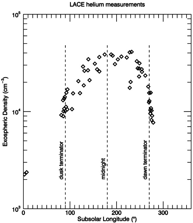
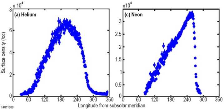
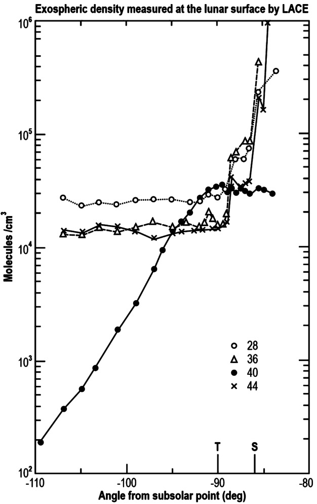
Volatiles and refractories represent the two end-members in the volatility range of species in any surface-bounded exosphere. Volatiles include elements that do not interact strongly with the surface, such as neon (detected on the Moon) and helium (detected both on the Moon and at Mercury), but also argon, a noble gas (detected on the Moon) that surprisingly adsorbs at the cold lunar nighttime surface. Refractories include species such as calcium, magnesium, iron, and aluminum, all of which have very strong bonds with the lunar surface and thus need energetic processes to be ejected into the exosphere. Here we focus on the properties of species that have been detected in the exospheres of inner Solar System bodies, specifically the Moon and Mercury, and how they provide important information to understand source and loss processes of these exospheres, as well as their dependence on variations in external drivers.

Keywords: Exosphere; Ions; Magnetosphere; Mercury; Moon; Neutrals; Refractories; Solar wind; Volatiles.

Fig. 1

Exospheric number densities for ⁴He measured at the lunar surface by the LACE mass spectrometer (Apollo 17) during nine lunations in 1972 and 1973. Subsolar longitudes are angles from the subsolar point. The two points at noon represent sporadic checks when the instrument was briefly turned on at noon. Adapted from Hoffman et al. (1973)

Fig. 2

Three different datasets (neutral helium measured in situ by LADEE/NMS: black diamonds; neutral helium measured remotely by LRO/LAMP: blue squares; solar wind alpha particles measured in situ by ARTEMIS/ESA: red line) show strongly correlated source rates between solar wind alpha particles and lunar exospheric helium. Vertical lines indicate times of full moon, when the geomagnetic tail effectively shields the Moon from the solar wind. Reproduced from Hurley et al. (2016)

Fig. 3

Peaks in exospheric source rate of ⁴⁰Ar measured by LACE (histogram) occurred soon after moonquakes recorded by the Apollo seismometers (red triangles). The black line is the argon exospheric loss rate. Adapted from Hodges (1977b)

Fig. 4

The diurnal profiles obtained four months apart (four lunations) by LACE in 1973. Measurements were made from dusk (90° subsolar longitude) to dawn (270° subsolar longitude). Adapted from Hodges (1975)

Fig. 5

Exospheric densities of ⁴⁰Ar measured at dawn (circles in top panel) are greatest above the western maria (middle panel), which are rich in KREEP elements, particularly ⁴⁰K (bottom panel), which is the radioactive parent of ⁴⁰Ar. Reproduced from Benna et al. (2015)

Fig. 6

Number densities of H₂ and ⁴⁰Ar measured by CHACE onboard Chandrayaan-1 from the ∼100 km altitude above the subsolar point to the surface close to the poles. Reproduced from Thampi et al. (2015)

Fig. 7

Surface densities for ⁴He (left) and ²⁰Ne (right) inferred from LADEE/NMS measurements at altitude. These panels show the different behavior of these two species, mainly attributed to their different scale height. Adapted from Benna et al. (2015)

Fig. 8

Methane number density measured by LADEE/NMS (colored lines) referenced to a common altitude of 12 km, around dawn. Black lines are exospheric simulations of methane. This figure shows the pronounced sunrise bulge in exospheric density, indicative of a species that condenses on the cold nighttime surface. Reproduced from Hodges (2016)

Fig. 9

LACE exospheric density at the surface from four masses. Masses 40 and 36 are interpreted to be argon. Mass 28 could be N₂ or CO. Mass 44 could be CO₂. This species is expected to adsorb at the lunar surface, so the lack of such a bulge at dawn is surprising. T indicates terminator; S indicates sunrise (delayed from the terminator by ∼8 hours because of the mountains to the West of the Taurus-Littrow valley). Adapted from Hoffman et al. (1973)

Fig. 10

Mechanism (recombinative desorption) for the creation of H and H₂ exospheres at the Moon or Mercury from solar wind protons and previously implanted H atoms. The diffusion rate depends on the temperature, whereas the implantation rate depends on the solar zenith angle. Reproduced from Tucker et al. (2019)

Fig. 11

Scheme of radon decay, with alpha particle energies pertaining to each product. The short half-life of radon makes it a useful species to constrain regions of active outgassing. Adapted from Lawson et al. (2005)

Fig. 12

(Left) Intensity at the surface over Mercury dawn determined from exponential fits to MESSENGER/MASCS limb profiles. Different Mercury years are indicated by different colors. (Center) Ca density in Mercury’s equatorial plane at Mercury true anomaly = 20° based on the simple dawn-centered model of Burger et al. (2014) ($T=70,000$ K, $\sigma =50$°, source rate $=3.7\times {10}^{23}$ s⁻¹). (Right) Comparison of the source rate determined at all true anomalies using the simple model shown in the center panel to the best-fit source rate at each true anomaly. The simple model works remarkably well. Adapted from Burger et al. (2014)

Fig. 13

Summary of MESSENGER/MASCS observations of Mg over two Mercury years. Top: MASCS observations (circles, color coded by Mercury year) over a Mg/Si elemental weight ratio composite map derived from MESSENGER/XRS measurements (Weider et al. 2015). Middle: temperature fit (using the model of Chamberlain 1963) to MASCS observations. It shows how the temperature from the emission lines (4,000–8,000 K) is independent on the year. Bottom: the retrieved production rate of Mg. It shows how observations in red (years when the Mg-rich terrain is exposed at dawn at perihelion) are consistent with a higher production rate than observations in blue (years when the terrain antipodal to the Mg-rich terrain is exposed at dawn at the perihelion). Adapted from Merkel et al. (2018)

Fig. 14

Line-of-sight tangent altitude profiles of Mn, Al, and Ca detected by MESSENGER/MASCS (spacecraft motion during the measurement of these profiles means they are not strictly radial profiles). The peculiar altitude profile of Mn, different from that of Ca⁺ or Al even though observed with similar geometry, when coupled with the timing in Mercury’s true anomaly angle, suggests that the Mn may be of cometary origin owing to a possible association with the comet 2P/Encke dust trail. Reproduced from Vervack et al. (2016)

Fig. 15

Mass spectrum of lunar ions detected by LADEE/NMS. Candidates for the substantial peak at m/q = 28 are ${\mathrm{N}}_2^{+}$, Si⁺, and CO⁺, with the latter one being the most plausible given the lower photo-ionization yields of the other two. Adapted from Halekas et al. (2015) with the addition of O⁺ signal at mass 16

Fig. 16

Mass spectrum of ions detected at Mercury by FIPS during MESSENGER’s first flyby (January 2008). Multiply charged ions (such as O⁺⁺, Si⁺⁺, and Mg⁺⁺) are observed mostly below $\text{m/q}\sim 12$, even though Fe⁺⁺ is observed at $\text{m/q}=28$. Dashed curves are Gaussian fits to the major peaks, and the solid blue curve is their sum. Adapted from Zurbuchen et al. (2008). Reprinted with permission from AAAS

Fig. 17

This composite image illustrates how ENA reflection (map in panel f) is predominantly correlated with lunar magnetic anomalies at the surface (see magnetic field at 30 km altitude from Lunar Prospector in panel e), rather than with topography (Clementine laser altimeter data in panel a), surface composition (Lunar Prospector gamma-ray spectrometer measurements of Fe and Th in panels b and c, respectively), or albedo (Clementine spectral reflectance mosaic at 750 nm in panel d). ENAs are therefore a useful tool for studying the exosphere-surface interaction, particularly on magnetic anomalies. Adapted from Vorburger et al. (2015)

References

1. A’Hearn M.F., Feldman P.D. Water vaporization on Ceres. Icarus. 1992;98(1):54–60. doi: 10.1016/0019-1035(92)90206-M. - DOI
1. Altwegg K., Balsiger H., Calmonte U., Hässig M., Hofer L., Jäckel A., et al. In situ mass spectrometry during the Lutetia flyby. Planet. Space Sci. 2012;66(1):173–178. doi: 10.1016/j.pss.2011.08.011. - DOI
1. Andrews G.B., et al. The energetic particle and plasma spectrometer instrument on the MESSENGER spacecraft. Space Sci. Rev. 2007;131:523–556. doi: 10.1007/s11214-007-9272-5. - DOI
1. Angelopoulos V. The ARTEMIS mission. Space Sci. Rev. 2011;165(1–4):3–25. doi: 10.1007/s11214-010-9687-2. - DOI
1. Arnold J.R. Ice in the lunar polar regions. J. Geophys. Res., Solid Earth (1978–2012) 1979;84(B10):5659–5668. doi: 10.1029/JB084iB10p05659. - DOI
LinkOut - more resources