The evolution of the solar wind

Abstract

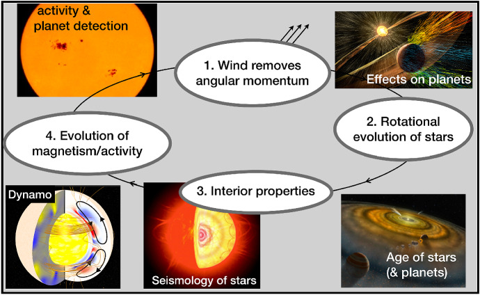
How has the solar wind evolved to reach what it is today? In this review, I discuss the long-term evolution of the solar wind, including the evolution of observed properties that are intimately linked to the solar wind: rotation, magnetism and activity. Given that we cannot access data from the solar wind 4 billion years ago, this review relies on stellar data, in an effort to better place the Sun and the solar wind in a stellar context. I overview some clever detection methods of winds of solar-like stars, and derive from these an observed evolutionary sequence of solar wind mass-loss rates. I then link these observational properties (including, rotation, magnetism and activity) with stellar wind models. I conclude this review then by discussing implications of the evolution of the solar wind on the evolving Earth and other solar system planets. I argue that studying exoplanetary systems could open up new avenues for progress to be made in our understanding of the evolution of the solar wind.

Keywords: Solar wind; Stars: activity, magnetism, rotation; Stellar winds and outflows; Stellar winds: observations and models.

Fig. 1

The big picture: evolution of winds of cool dwarf stars. As the star ages, its rotation and magnetism decrease, causing also a decrease in angular momentum removal. In the images, I highlight some of the areas to which wind-rotation-magnetism interplay is relevant. Image reproduced with permission from Vidotto (2016a)

Fig. 2

An overview of mass-loss rates (colour coded) in the cool-star HR diagram. Winds of cool stars evolve from hot ($\sim {10}^6$ K) and tenuous (‘hot corona’) to cold ($\sim {10}^4$ K) and denser (‘no corona’). Evolved low-mass stars that show weak or sporadic signatures of a hot corona are denoted ‘warm/hybrid’. The zero-age main sequence is shown by the grey line. Image reproduced with permission from Cranmer and Winebarger (2019), copyright by Annual Reviews

Fig. 3

Sketch of the ISM (left) interacting with a stellar wind (right) and giving rise to an astrosphere, which is surrounded by a hydrogen wall and possibly a bow shock. The hydrogen wall, which is an enhancement of hydrogen density, is located between the bow shock and the astropause. Figure adapted from Ó Fionnagáin (2020)

Fig. 4

Summary of mass-loss rates for low-mass stars derived from the astrosphere method. For GK dwarfs (red filled circles), the mass-loss rate per unit surface area varies as a function of X-ray flux as $\propto F_X^{1.34}$ (shaded line). It has been suggested that active (and overall younger) stars with $F_X\gtrsim {10}^6\mathrm{erg}{\mathrm{s}}^{-1}{\mathrm{cm}}^{-2}$ would have reduced mass-loss rates, thus giving rise to a ‘wind dividing line’. Some new mass-loss rates measurements indicate that mass-loss rates of young Suns could actually remain large (cf. Sect. 3). Image reproduced with permission from Wood (2018), copyright by the author

Fig. 5

Predicted evolution of the radio flux with rotation, used as proxy for stellar age, for a number of solar-like stars. The spectra of all these stars have been normalised to 10 pc. Young stars, close-by, are the targets which would present the strongest radio flux. Figure adapted from Ó Fionnagáin et al. (2019)

Fig. 6

The formation of slingshot prominences occurs when in the ‘limit-cycle regime’. In this case, the site of prominence formation, i.e., on loop-tops at the corotation radius, occurs above the sonic point (the star is “unaware” that the prominence has formed and thus keeps loading it with stellar wind material) and below the Alfvén radius (beyond the Alfvén radius all magnetic field lines will be open). By observing slingshot prominences, one can estimate the rate at which mass is loaded into the loop tops and thus derive mass-loss rates of stellar winds. Image reproduced with permission from Jardine and Collier Cameron (2019), copyright by the authors

Fig. 7

Left: Number density of the wind of a solar-like star with a mass-loss rate of $2\times {10}^{-12}{M}_{\odot }{\mathrm{yr}}^{-1}$. A planet is considered to orbit at 0.02 au, with the observer looking towards the system from the negative x-direction. The dashed line shows the radio photosphere where 50% of a 30-MHz wind emission is produced. The hypothetical 30-MHz radio emission of this planet is increasingly more attenuated after the planet ingresses the radio photosphere and the attenuation peaks at orbital phase $\varphi =0.5$. Its emission is least attenuated at $\varphi =0$. Given that the position of the radio photosphere is linked to the stellar wind properties, monitoring of planetary radio emission could allow one to derive stellar wind properties. Right: The situation on the left panel only occurs if the plasma emission $f_p$ is below the cyclotron frequency $f_c$ of the planetary emission (white area). If the wind of the host star has a high mass-loss rate and the planet has a weak magnetic field, such that $f_p>f_c$, then the planetary radio emission cannot propagate through the wind of the host star (grey area). Detections of planetary radio emission can thus place an upper limit on the mass-loss rate of the star (Eq. 8). Note that the wind parameters used to produce this figure is based on models of the weak-lined T Tauri star V830 Tau. Images reproduced with permission from [left] Kavanagh and Vidotto (2020), copyright by the authors; and from [right] Vidotto and Donati (2017), copyright by ESO

Fig. 8

Summary of derived mass-loss rates for low-mass stars combining results from the different methods discussed in Sect. 2. The y-axis is given in solar values, i.e., ${\dot{M}}_{\odot }/R_{\odot }^2$, with ${\dot{M}}_{\odot }=2\times {10}^{-14}{M}_{\odot }{\mathrm{yr}}^{-1}$. Colour indicates the method used in the derivation: blue for exoplanets, orange for astrospheres, green for prominences, black for the Sun at minimum/maximum of its sunspot cycle. Grey arrows indicate upper limits, which are mostly derived from radio observations. The solid line is a power-law fit through the larger circles. The smaller symbols are either evolved stars or M dwarfs, which were not included in the fit and neither were the stars for which only upper limits exist (arrows). The values used in this plot were compiled from the following works: Drake et al. (1993); Lim et al. (1996); Gaidos et al. (2000); Wood et al. (2001, 2002, 2005a, 2014); Wood and Linsky (2010); Wood (2018); Wargelin and Drake (2002); Bourrier et al. (2013); Kislyakova et al. (2014); Fichtinger et al. (2017); Vidotto and Bourrier (2017); Vidotto and Donati (2017); Jardine and Collier Cameron (2019); Finley et al. (2019); Ó Fionnagáin et al. (2021)

Fig. 9

The mass-loss rate of the solar wind (solid black line) has a small variation during the solar cycle. The green line is the estimated open magnetic flux of the solar wind. Data shows cycles 23 and 24. Image adapted from Finley et al. (2019)

Fig. 10

Solar wind variations during its magnetic cycle. Left: At cycle minimum (cycle 22), the solar magnetic field resembles an aligned dipole and the solar wind shows a bimodal velocity distribution, with faster streams emerging from high-latitude coronal holes and slower streams remaining in the equatorial plane. Right: At cycle maximum (cycle 23), the solar magnetic field geometry is more complicated, which is reflected in the solar wind velocity distribution. The background image shows a zoom-in of the solar corona extending out to a few solar radii, while the polar plot shows the solar wind speed measured by Ulysses at several au from the Sun. Colour indicates the magnetic field polarity (red for outward, blue for inward). Images reproduced with permission from McComas et al. (2003), copyright by AGU

Fig. 11

An evolutionary mass loss sequence. Predictions on how the solar wind mass-loss rate would have been in the past. These power-laws are discussed in the text and here they are normalised to match the present-day solar wind mass-loss rates. Note that the power-laws carry large uncertainties in their slope, which are not illustrated in this figure. The proxy for the young Sun at 2 Myr, V830 Tau, is shown on the left of the plot. The question mark here emphasises that, from observational studies, we are not sure how the solar wind has evolved from the end of the pre-main sequence/beginning of the main sequence, until today. The mass-loss rate saturation discussed in Johnstone et al. (2015a) is shown schematically by the horizontal line

Fig. 12

Top: The reconstructed stellar magnetic field using the ZDI technique for the F-type star $\tau$ Boo (Fares et al. 2009). Middle: Synoptic map of the Sun plotted with data from Gosain et al. (2013). The solar map, due to its increased resolution, shows a lot more structure in the surface magnetic field. Bottom: To compare the solar map with the stellar map, I filtered out the small-scale magnetic field structure of the Sun (Vidotto 2016b). At the top of each panel, I show the maximum harmonic order ${\ell }_{max}$ for each map and its typical spatial resolution

Fig. 13

Magnetic flux relations for low-mass stars. The columns on the left show measurements of Zeeman broadening fields and the right columns present measurements of ZDI fields. The top row shows magnetic field as a function of Rossby number and the bottom row shows X-ray luminosity as a function of magnetic flux. a Crosses are Sun-like stars, circles are M-type of spectral class M6 and earlier, red squares are late M dwarfs. I performed a rough computation of the power-law dependence with Ro for the unsaturated stars: $⟨|B_I|⟩\propto {\mathrm{Ro}}^{-1.41\pm 0.22}$. b, d Different symbols correspond to different ZDI surveys (open circles are the late and mid M dwarfs, not considered in the fits). c Dots are for the quiet Sun, squares for X-ray bright points, diamonds for solar active regions; pluses for solar-disc averages, crosses for G, K, and M dwarfs, and circles are for T Tauri stars. Solid lines shown in the last three panels are power-law fits. Images reproduced with permission from a Reiners (2012); b, d Vidotto et al. (2014a); c Pevtsov et al. (2003), copyright by AAS

Fig. 14

The average unsigned large-scale magnetic field decays with age as $t^{-0.655}$. This is a similar trend as seen in ${\Omega }_{\star }(t)$ (Eq. 22). Different symbols correspond to different ZDI surveys. Note that the Sun is represented at minimum and maximum phases of its magnetic cycle. Typical error bars are indicated on the bottom left. Image reproduced with permission from Vidotto et al. (2014a), copyright by the authors

Fig. 15

Rotational evolution from solar-mass stars. Pluses are observations of rotation rates of open cluster stars, circle is the present-day Sun and the rectangle shows the velocity dispersion of old disc field stars. The grey shaded bars in a highlight the velocity dispersion at each age. The red, green, and blue diamonds represent the 25th, 50th, and 90th rotational percentiles, respectively. In b, models are over-plotted to these observations. Image adapted and reproduced with permission from Gallet and Bouvier (2015), copyright by ESO

Fig. 16

The X-ray-rotation activity relation shows how the normalised X-ray luminosity $R_X=L_X/L_{\mathrm{bol}}$ varies as a function of Rossby number (fast rotators on the left, slow rotators on the right of the x axis). Image adapted from Reiners et al. (2014), copyright by AAS

Fig. 17

Evolution of high-energy irradiation of solar type stars. Left: The observed evolution of high-energy flux at a given orbital distance at different bands. Right: The X-ray (left axis) and extreme ultraviolet (right axis) luminosities derived from rotational evolution tracks (e.g., Fig. 15) as a function of stellar age. Images reproduced with permission from (left) Ribas et al. (2005), copyright by AAS; and (right) Tu et al. (2015), copyright by ESO

Fig. 18

Solar XUV flux as a function of the surface magnetic flux. Open symbols represent the surface magnetic flux calculated directly from HMI synoptic maps. Filled symbols represent the Sun-as-a-star, where only harmonics up to order ${\ell }_{max}=10$ were used. Colours show temporal evolution with darkest colour corresponding to year 2010.5 and lightest colour to year 2019.5 (solar cycle 24). The solid lines show power-law fits to the data. Further discussion is shown in Hazra et al. (2020)

Fig. 19

Left: The output kinetic luminosity ($\dot{M}{u}_r^2/2$, y-axis) of stellar winds increases with the input wave luminosity (x-axis) at the photosphere (subscript ‘0’). Different values of magnetic field strengths are shown by the different symbols. Curves of constant ratios between y-axis and x-axis (labeled $c_E$) are shown by the solid lines. Right: The same as the left panel, but instead of the input wave luminosity, the x-axis now shows the wave luminosity as measured at the transition region (top of the chromosphere, subscript ‘tc’). Images reproduced with permission from Suzuki et al. (2013), copyright by ASJ

Fig. 20

a Magnetic field line extrapolations, assuming a potential field source surface model. The surface magnetic field is derived from ZDI observations (Donati et al. 2008). The potential field model assumes the stellar magnetic field is in its minimum energy state. b The field lines are stressed after interaction with stellar wind flow. Based on the simulations presented in Vidotto et al. (2014b)

Fig. 21

Left: Velocity of the simulated stellar wind (in km/s) of the planet-hosting star HD 189733, at the position of the orbit of the exoplanet HD 189733b. The blue circles denote an inward component of the magnetic field and the green diamonds denote an outward component. The computed free-free X-ray emission of the coronal wind is shown in the background. The structure that the stellar magnetic field imposes on the X-ray corona is correlated with the structure of the stellar wind. Right: Histogram of wind velocities for 3D MHD simulations of the wind of the young solar-like star HII 296. Three velocity components related to magnetic field geometry can be identified: a slow one at 250 km/s emanating from helmet streamers, a fast component at 500 km/s (dashed-magenta line) from expanded flux tubes and an intermediate velocity of 400 km/s. Images reproduced with permission from [left] Llama et al. (2013), copyright by the authors; and from [right] Réville et al. (2016), copyright by AAS

Fig. 22

Solutions to the momentum equation of an isothermal wind for different wind temperatures. The sonic points are marked by the filled circles, in the zoomed-in panel on the right

Fig. 23

Left: initial setup of the split monopole. Right: the trailing spiral structure that is created once stellar rotation is set

Fig. 24

The specific angular momentum of the solar wind calculated by Weber and Davis (1967). The sum of these two terms is constant with distance and simplifies to $\mathcal{L}={\Omega }_{\star }{r}_A^2$ (see Eqs. 58 and 60), where $r_A$ is the distance to the Alfvén point. Image reproduced with permission, copyright by AAS

Fig. 25

In 3D, the Alfvén radius takes the form of an Alfvén surface (grey surface). Because of the complex stellar surface magnetic field geometry (shown by the colour bar), the Alfvén surface can be highly asymmetric. Image reproduced with permission from Vidotto et al. (2014b), copyright by the authors

Fig. 26

Evolution of the Galactic cosmic ray spectrum at Earth’s orbit. The figure above shows Galactic cosmic ray differential intensity as a function of their kinetic energies. The different curves refer to different solar rotation rates normalised to present-day value (here denoted by ${\Omega }_0$). Each curve thus represents a different age, which ranges from about 6–1 Gyr from the top to the bottom dashed lines. The black dashed line is thus for the present-day value (1${\Omega }_0$) at Earth’s orbit. The black solid line is the cosmic ray spectrum at the local interstellar medium. Cosmic rays are suppressed (i.e., modulated) as they travel through the solar wind and, given the solar wind evolution, the spectrum of Galactic cosmic rays at Earth changes with time. The red lines and red shaded area represent a range of rotation values that the Sun could have had at 600 Myr. Image reproduced with permission from Rodgers-Lee et al. (2020), copyright by the authors

References

1. Aarnio AN, Stassun KG, Hughes WJ, McGregor SL. Solar flares and coronal mass ejections: a statistically determined flare flux–CME mass correlation. Sol Phys. 2011;268(1):195–212. doi: 10.1007/s11207-010-9672-7. - DOI
1. Aarnio AN, Matt SP, Stassun KG. Mass loss in pre-main-sequence stars via coronal mass ejections and implications for angular momentum loss. ApJ. 2012;760(1):9. doi: 10.1088/0004-637X/760/1/9. - DOI
1. Airapetian VS, Usmanov AV. Reconstructing the solar wind from its early history to current epoch. ApJ. 2016;817(2):L24. doi: 10.3847/2041-8205/817/2/L24. - DOI
1. Airapetian VS, Barnes R, Cohen O, Collinson GA, Danchi WC, Dong CF, Del Genio AD, France K, Garcia-Sage K, Glocer A, Gopalswamy N, Grenfell JL, Gronoff G, Güdel M, Herbst K, Henning WG, Jackman CH, Jin M, Johnstone CP, Kaltenegger L, Kay CD, Kobayashi K, Kuang W, Li G, Lynch BJ, Lüftinger T, Luhmann JG, Maehara H, Mlynczak MG, Notsu Y, Osten RA, Ramirez RM, Rugheimer S, Scheucher M, Schlieder JE, Shibata K, Sousa-Silva C, Stamenković V, Strangeway RJ, Usmanov AV, Vergados P, Verkhoglyadova OP, Vidotto AA, Voytek M, Way MJ, Zank GP, Yamashiki Y. Impact of space weather on climate and habitability of terrestrial-type exoplanets. Int J Astrobiol. 2020;19(2):136–194. doi: 10.1017/S1473550419000132. - DOI
1. Alfvén H. Magneto hydrodynamic waves, and the heating of the solar corona. MNRAS. 1947;107:211. doi: 10.1093/mnras/107.2.211. - DOI
LinkOut - more resources