Spatial subsidies drive sweet spots of tropical marine biomass production

Abstract

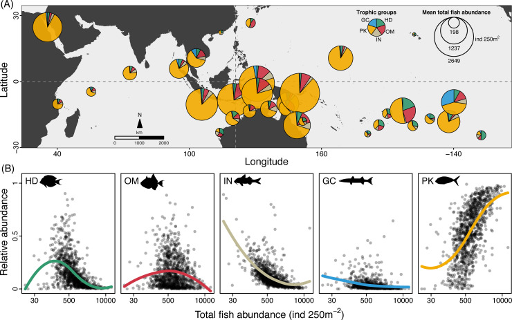
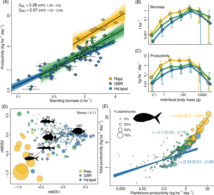
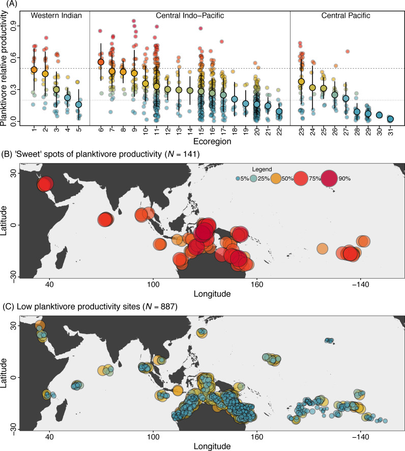
Spatial subsidies increase local productivity and boost consumer abundance beyond the limits imposed by local resources. In marine ecosystems, deeper water and open ocean subsidies promote animal aggregations and enhance biomass that is critical for human harvesting. However, the scale of this phenomenon in tropical marine systems remains unknown. Here, we integrate a detailed assessment of biomass production in 3 key locations, spanning a major biodiversity and abundance gradient, with an ocean-scale dataset of fish counts to predict the extent and magnitude of plankton subsidies to fishes on coral reefs. We show that planktivorous fish-mediated spatial subsidies are widespread across the Indian and Pacific oceans and drive local spikes in biomass production that can lead to extreme productivity, up to 30 kg ha-1 day-1. Plankton subsidies form the basis of productivity "sweet spots" where planktivores provide more than 50% of the total fish production, more than all other trophic groups combined. These sweet spots operate at regional, site, and smaller local scales. By harvesting oceanic productivity, planktivores bypass spatial constraints imposed by local primary productivity, creating "oases" of tropical fish biomass that are accessible to humans.

Fig 1. Neither fishers nor fishes are randomly distributed across reef scapes.

(A) By searching and concentrating on the best, “sweetest” fishing spots, fishers intend to maximise their catch relative to effort or risk. (B) Here, we show that plankton subsidies can, and do, underpin the occurrence of “sweet spots” of fish productivity on coral reefs at a global scale, sustaining productive assemblage not only of planktivorous reef fishes, but also of their predators. Photo credits: (A) João Luiz Gasparini, National Geographic Society; (B) Yen Yi Lee, Coral Reef Image Bank.

Fig 2. The trophic structure of Indo-Pacific reef fish assemblages.

(A) Reef fish abundances across 32 ecoregions, from the Western Indian to the Central Pacific, were clearly dominated by planktivores (in yellow). Pies indicate proportional mean abundance for ecoregions from the RLS dataset [41]. (B) From the 5 reef fish trophic groups evaluated, PK are the only one where proportional abundance increases as total fish abundance increases. Dots represent mean abundances for each of the 1,035 sites, and trend lines are polynomial regression fits (LOESS smoothers). Note the log-scale in the x-axis of panels in (B). Map source: Natural Earth via the maps and mapdata packages in R. Numerical values underlying this figure are provided in “Morais_et_al_Fig 02_DataS1.R,” available from https://doi.org/10.5281/zenodo.5540102. GC, generalised macrocarnivores; HD, herbivores/detritivores; IN, invertivores; OM, omnivores; PK, planktivores; RLS, Reef Life Survey.

Fig 3. Distinct reef fish productivity–biomass relationships among the 3 locations examined arise from similar size structures but different trophic structures.

(A) Regression lines for all locations had a similar slope but different intercepts. Dots are the bootstrap medians for survey areas, and segments delimit the 95% bootstrap quantile intervals (see Methods). Coloured lines represent 500 draws from the Bayesian posterior distributions and black lines represent the posterior medians. (B) Biomass and (C) productivity size distributions, with median (dots) and 90% bootstrap quantile intervals. (D) An nMDS biplot showing trophic groups as vectors and survey areas as circles scaled proportionally to total fish productivity. (E) Relationship between the productivity of PK and total fish productivity in the 3 locations. Trendlines depict 300 bootstrapped Pearson’s correlation r values (coloured lines) and median r (dashed lines) back calculated from standardised variables to productivity units (see Methods and S3 Fig) for each location. Circles are survey areas and are scaled proportionally to relative PK productivity. To improve clarity, only 60 randomly selected survey areas out of 284 are depicted for Ha’apai in (A) and (E). The same plots with all data points unscaled are available as S2 Fig. Note the log-scale in the axes of panels (A), (B), (C), and (E). Numerical values underlying this figure are provided in “Morais_et_al_Fig 03_FigS2.R,” available from https://doi.org/10.5281/zenodo.5540102. GBR, Great Barrier Reef; GC, generalised carnivores; HD, herbivores/detritivores; IN, invertivores; nMDS, nonmetric multidimensional scaling; OM, omnivores; PK, planktivores.

Fig 4. The geography of planktivore contributions to fish productivity on Indo-Pacific coral reefs.

(A) The distribution of predicted proportional planktivore productivity for 1,028 sites in 31 ecoregions distributed across the Western Indian, Central Indo-Pacific, and Central Pacific Oceans. Larger circles are means, and intervals represent standard deviations. Dashed line marks the “sweet spot” threshold (50% or more of total productivity), and the dotted line marks the expected proportion comprised by any single trophic group (20% of total productivity). Region labels are in the S1 Data. (B) The geographic location of “sweet spots” (>50% of total) and (C) low (<50% of total) planktivore proportional productivity. In all plots, colours range from low (blue shades) to high (red shades) predicted relative planktivorous fish productivity. Map source: Natural Earth via the maps and mapdata packages in R. Numerical values underlying this figure are provided in “Morais_et_al_Fig 04.R,” available from https://doi.org/10.5281/zenodo.5540102.

References

1. Loreau M, Mouquet N, Holt RD. Meta-ecosystems: a theoretical framework for a spatial ecosystem ecology. Ecol Lett. 2003;6:673–9. doi: 10.1046/j.1461-0248.2003.00483.x - DOI
1. Polis GA, Anderson WB, Holt RD. Toward an Integration of Landscape and Food Web Ecology: The Dynamics of Spatially Subsidized Food Webs. Annu Rev Ecol Syst. 1997;2:289–316.
1. Polis GA, Hurd SD. Allochthonous Input Across Habitats, Subsidized Consumers, and Apparent Trophic Cascades: Examples from the Ocean-Land Interface. In: Polis GA, Winemiller KO, editors. Food Webs. Boston, MA: Springer US; 1996. p. 275–285. doi: 10.1007/978-1-4615-7007-3_27 - DOI
1. Polis GA, Hurd SD. Extraordinarily high spider densities on islands: flow of energy from the marine to terrestrial food webs and the absence of predation. Proc Natl Acad Sci. 1995;92:4382–6. doi: 10.1073/pnas.92.10.4382 - DOI - PMC - PubMed
1. Trebilco R, Baum JK, Salomon AK, Dulvy NK. Ecosystem ecology: size-based constraints on the pyramids of life. Trends Ecol Evol. 2013;28:423–31. doi: 10.1016/j.tree.2013.03.008 - DOI - PubMed
Publication types