Ankle muscles drive mediolateral center of pressure control to ensure stable steady state gait

Abstract

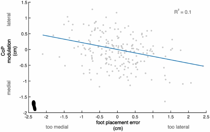
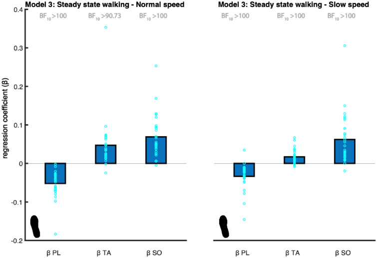
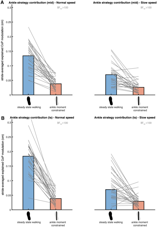
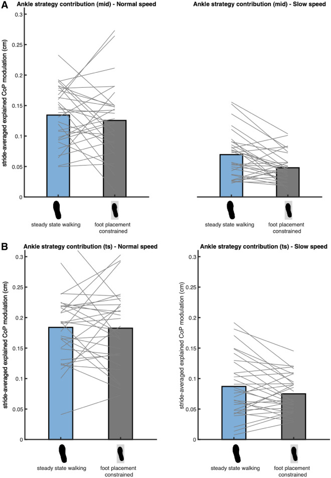
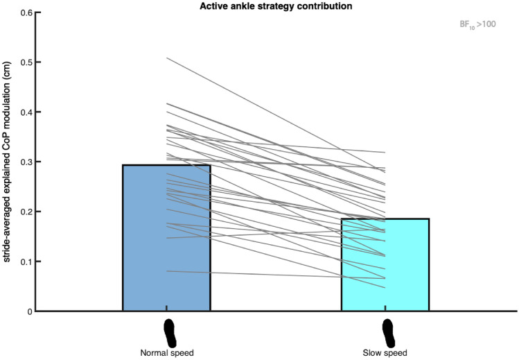
During steady-state walking, mediolateral gait stability can be maintained by controlling the center of pressure (CoP). The CoP modulates the moment of the ground reaction force, which brakes and reverses movement of the center of mass (CoM) towards the lateral border of the base of support. In addition to foot placement, ankle moments serve to control the CoP. We hypothesized that, during steady-state walking, single stance ankle moments establish a CoP shift to correct for errors in foot placement. We expected ankle muscle activity to be associated with this complementary CoP shift. During treadmill walking, full-body kinematics, ground reaction forces and electromyography were recorded in thirty healthy participants. We found a negative relationship between preceding foot placement error and CoP displacement during single stance; steps that were too medial were compensated for by a lateral CoP shift and vice versa, steps that were too lateral were compensated for by a medial CoP shift. Peroneus longus, soleus and tibialis anterior activity correlated with these CoP shifts. As such, we identified an (active) ankle strategy during steady-state walking. As expected, absolute explained CoP variance by foot placement error decreased when walking with shoes constraining ankle moments. Yet, contrary to our expectations that ankle moment control would compensate for constrained foot placement, the absolute explained CoP variance by foot placement error did not increase when foot placement was constrained. We argue that this lack of compensation reflects the interdependent nature of ankle moment and foot placement control. We suggest that single stance ankle moments do not only compensate for preceding foot placement errors, but also assist control of the subsequent foot placement. Foot placement and ankle moment control are 'caught' in a circular relationship, in which constraints imposed on one will also influence the other.

Figure 1

LesSchuh. Shoe with ankle moment constraint (width of the ridge is 1 cm). Figure as published in.

Figure 2

Local foot coordinate system. Based on digitized anatomical landmarks a model of this example participant was constructed. The full model has been depicted on the left. Magnified is the local coordinate system (X, Y, Z) of the right foot with its anatomical landmarks (light blue circles). The local coordinate system was constructed based on the medial (1) and lateral (2) malleoli, the calcaneus (3) and the second toe tip (4). The origin of the constructed coordinate system lies at the estimated foot’s CoM position (5). The red, dark blue and green lines represent respectively the local vertical (Z), forward (X) and mediolateral axes (Y). We defined our mediolateral CoP shift along the anatomical Y-axis in green. Note that in this figure this mediolateral axis points positively to medial, yet in our analysis we flipped the sign to define a lateral shift as positive and a medial shift as negative. This figure was created using Matlab 2021a (https://www.mathworks.com/products/matlab.html) and Adobe Illustrator CC 2018 (https://www.adobe.com/nl/products/illustrator.html).

Figure 3

Mean regression coefficients of the ankle strategy model (2). The predictors (β) are the foot placement error at mid-swing and terminal swing. The foot print represents the steady-state walking condition (see Table 1). The light blue circles represent individual data points. The negative relationship shows ankle moments accommodate for stepping inaccuracies, by shifting the CoP in the opposite direction. The Bayes factors (BF₁₀) represent the degree of evidence supporting the regression coefficients to be different from zero. This figure was created using Matlab 2021a (https://www.mathworks.com/products/matlab.html) and Adobe Illustrator CC 2018 (https://www.adobe.com/nl/products/illustrator.html).

Figure 4

Relationship between foot placement error and subsequent CoP shift. Example of one participant, demonstrating a negative relationship between CoP modulation (ankle moment control) and foot placement error. The blue line represents the fitted model (2) and the data points represent individual (right and left) steps. The foot print represents the steady-state walking condition (see Table 1). Compared to the other participants, this participant demonstrated a relatively high relative explained variance (R² = 0.1). This figure was created using Matlab 2021a (https://www.mathworks.com/products/matlab.html) and Adobe Illustrator CC 2018 (https://www.adobe.com/nl/products/illustrator.html).

Figure 5

Mean regression coefficients of the muscle model (3). The predictors (β) are the peroneus longus (PL), tibialis anterior (TA) and soleus (SO) muscles’ activity. The foot print represents the steady-state walking condition (see Table 1). The light blue circles represent individual data points. The Bayes factors (BF₁₀) represent the degree of evidence supporting the regression coefficients to be different from zero. This figure was created using Matlab 2021a (https://www.mathworks.com/products/matlab.html) and Adobe Illustrator CC 2018 (https://www.adobe.com/nl/products/illustrator.html).

Figure 6

Mean absolute explained variance of the ankle strategy model (2). For normal (left) and slow (right) walking speeds panels A and B depict respectively the absolute explained variances for the foot placement error at mid- and terminal swing. Blue and red bars represent the steady-state walking and ankle moment constrained conditions respectively. In this figure the absolute explained variance is expressed as the square root of the stride averaged explained variance, as a reflection of the magnitude of the average explained CoP shift in centimeters. The grey lines connect individual data points. The Bayes factors (BF₁₀) denote the degree of evidence for a decreased absolute explained variance in the ankle moment constrained condition, as compared to steady-state walking. This figure was created using Matlab 2021a (https://www.mathworks.com/products/matlab.html) and Adobe Illustrator CC 2018 (https://www.adobe.com/nl/products/illustrator.html).

Figure 7

Mean absolute explained variance of the ankle strategy model (2). For normal (left) and slow (right) walking speeds panels A and B depict respectively the absolute explained variances for the foot placement error at mid- and terminal swing. Blue and grey bars represent the steady-state walking and foot placement constrained conditions respectively. In this figure the absolute explained variance is expressed as the square root of the stride averaged explained variance, as a reflection of the magnitude of the average explained CoP shift in centimeters. The grey lines connect individual data points. As the best model did not include the factor Condition, no Bayes factors have been presented. This figure was created using Matlab 2021a (https://www.mathworks.com/products/matlab.html) and Adobe Illustrator CC 2018 (https://www.adobe.com/nl/products/illustrator.html).

Figure 8

Mean absolute explained variance of the muscle model (3). Blue and light blue bars represent respectively the absolute explained variance at normal and slow walking speed. In this figure the absolute explained variance is expressed as the square root of the stride averaged explained variance, as a reflection of the magnitude of the average explained CoP shift in centimeters. The foot print represents the steady-state walking condition (see Table 1). The grey lines connect individual data points. The Bayes factor (BF₁₀) denotes the degree of evidence for a lower absolute explained variance at slow as compared to at normal walking speed. This figure was created using Matlab 2021a (https://www.mathworks.com/products/matlab.html) and Adobe Illustrator CC 2018 (https://www.adobe.com/nl/products/illustrator.html).

References

1. Rankin BL, Buffo SK, Dean JC. A neuromechanical strategy for mediolateral foot placement in walking humans. J. Neurophysiol. 2014;112:374–383. doi: 10.1152/jn.00138.2014. - DOI - PMC - PubMed
1. Hof A, Vermerris S, Gjaltema W. Balance responses to lateral perturbations in human treadmill walking. J. Exp. Biol. 2010;213:2655–2664. doi: 10.1242/jeb.042572. - DOI - PubMed
1. Mahaki M, Bruijn SM, Van Dieën JH. The effect of external lateral stabilization on the use of foot placement to control mediolateral stability in walking and running. PeerJ. 2019;7:e7939. doi: 10.7717/peerj.7939. - DOI - PMC - PubMed
1. Bruijn SM, van Dieën JH. Control of human gait stability through foot placement. J. R. Soc. Interface. 2018;15:20170816. doi: 10.1098/rsif.2017.0816. - DOI - PMC - PubMed
1. Hof AL. The equations of motion for a standing human reveal three mechanisms for balance. J. Biomech. 2007;40:451–457. doi: 10.1016/j.jbiomech.2005.12.016. - DOI - PubMed
Publication types