Multiscale Computational Model Predicts Mouse Skin Kinematics Under Tensile Loading

Abstract

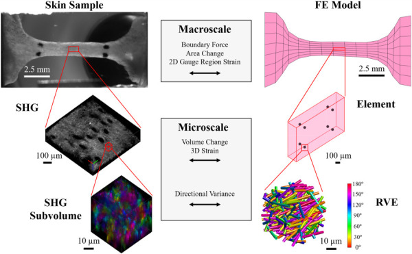
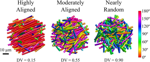
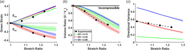
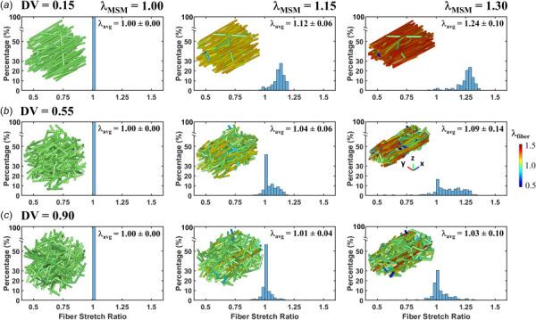
Skin is a complex tissue whose biomechanical properties are generally understood in terms of an incompressible material whose microstructure undergoes affine deformations. A growing number of experiments, however, have demonstrated that skin has a high Poisson's ratio, substantially decreases in volume during uniaxial tensile loading, and demonstrates collagen fiber kinematics that are not affine with local deformation. In order to better understand the mechanical basis for these properties, we constructed multiscale mechanical models (MSM) of mouse skin based on microstructural multiphoton microscopy imaging of the dermal microstructure acquired during mechanical testing. Three models that spanned the cases of highly aligned, moderately aligned, and nearly random fiber networks were examined and compared to the data acquired from uniaxially stretched skin. Our results demonstrate that MSMs consisting of networks of matched fiber organization can predict the biomechanical behavior of mouse skin, including the large decrease in tissue volume and nonaffine fiber kinematics observed under uniaxial tension.

Keywords: biomechanics; collagen; dermis; fiber networks; multiphoton microscopy; nonaffine.

Fig. 1

Multiscale experiment and model. Experimental data acquired at the macro- and microscales were used to construct image-based models and assess their predictions. The models consist of a finite element mesh that approximates the geometry of the skin sample and a set of 3D collagen fiber networks that represent collagen fiber properties, such as directional variance (DV), measured from SHG subvolumes. The collagen networks are contained within representative volume elements (RVEs) centered at the integration points of the elements. Model predictions of the experiment are then compared with experimental data. At the macroscale, the experimental data available includes the force on the boundary, the change in sample area, and the two-dimensional (2D) strain measured at the center of the gauge region from the four fiducial markers. At the microscale, the experimental data available include the volume change, 3D strain, and DV of subregions within the SHG image volume. Model comparisons at the microscale are made with the central element indicated, which corresponds to the location of the imaging area in the sample. The red cube depicted shows a subvolume (40 μm a side) and the corresponding RVE of the same size in the model. Both the fibers in the subvolume and in the RVE are color coded according to orientation with respect to the axis of stretch.

Fig. 2

Microscale RVE fiber network cases. To evaluate the effect of microstructural organization on model behavior, three types of networks were investigated: a highly aligned fiber network (DV = 0.15), a moderately aligned network that matched the initial directional variance obtained experimentally (DV = 0.55), and a random network (DV = 0.90). The principal directions and densities of the fiber networks also closely approximated experimental values. The color bar indicates the fiber orientation relative to the axis of stretch.

Fig. 3

Macroscale comparison of model and sample mechanics. (a) Force versus stretch ratio for all simulations. Parameters for the moderately aligned DV = 0.55 model (red) were selected to match the experiment loading curve (black), which displayed typical nonlinear behavior. Depicted are the average and standard deviation of n = 5 simulations per network type. (b) A representative simulation for the DV = 0.55 model showing area change and marker movement in response to stretch. Cyan circles represent the locations on the markers that were tracked in the experiment and the magenta Xs represent the equivalent location in the model. As the sample stretched, the large inward contraction in the gauge region was replicated in the simulation. The model, however, did not contract inward as much in the grip regions and in the transition zones. (c) Comparison of the 2D green strain calculated at the midpoint of the four fiduciary markers shows that the models overestimated E_xx and underestimated E_yy.

Fig. 4

Microscale comparison of model simulation with experiment. Model predictions of (a) Green strain in the x- and y-directions and (b) volume in the central element for each model. The moderately aligned DV = 0.55 model matched the strain and volume measured in the SHG volume well. (c) DV decreased with stretch in the experiment and in all three network models as a function of network capacity for fiber realignment.

Fig. 5

Fiber network behavior. Representative fiber networks in the central element from the (a) highly aligned (DV = 0.15), (b) moderately aligned (DV = 0.55), and (c) random (DV = 0.90) models demonstrate fiber reorganization with an increase in stretch. Fibers are colored with the stretch ratio generated during mechanical loading. A corresponding histogram shows the distribution of fiber stretches along with the average and standard deviation. (a) DV = 0.15 (b) DV = 0.55 (c) DV = 0.90)

Fig. 6

Multiscale fiber reorganization. Change in initial directional variance (ΔDV) and average direction of fiber alignment in the x–y plane. Representative simulations for (a) highly aligned (DV = 0.15), (b) moderately aligned (DV = 0.55), and (c) random (DV = 0.90) models. A negative ΔDV corresponds to a region that increased in alignment. Average fiber direction is depicted with a red line. The magnitude of the line corresponds to DV. The greatest change in ΔDV occurs in the gauge region of the nearly isotropic model, whereas the greatest degree of alignment occurs in the highly aligned model.(a) DV = 0.15 (b) DV = 0.55 (c) DV = 0.90)

References

1. Kanitakis, J. , 2002, “ Anatomy, Histology and Immunohistochemistry of Normal Human Skin,” Eur. J. Dermatol., 12(4), pp. 390–399.https://pubmed.ncbi.nlm.nih.gov/12095893/ - PubMed
1. Yousef, H. , Alhajj, M. , and Sharma, S. , 2020, “ Anatomy, Skin (Integument), Epidermis,” StatPearls, Treasure Island, FL. - PubMed
1. Phillip, J. M. , Aifuwa, I. , Walston, J. , and Wirtz, D. , 2015, “ The Mechanobiology of Aging,” Annu. Rev. Biomed. Eng., 17(1), pp. 113–141.10.1146/annurev-bioeng-071114-040829 - DOI - PMC - PubMed
1. Pissarenko, A. , and Meyers, M. A. , 2020, “ The Materials Science of Skin: Analysis, Characterization, and Modeling,” Prog. Mater. Sci., 110, p. 100634.10.1016/j.pmatsci.2019.100634 - DOI
1. Blair, M. J. W. A. E. , Balachandran, K. , and Quinn, K. P. , 2019, “ Fast-Acquisition Quantitative Polarized Light Imaging for Mechanical Testing of Collagenous Tissues,” Biomedical Engineering Society Meeting, Philadelphia, PA, Oct. 15–19.
Publication types