Next-generation ensemble projections reveal higher climate risks for marine ecosystems

Abstract

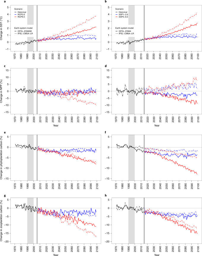
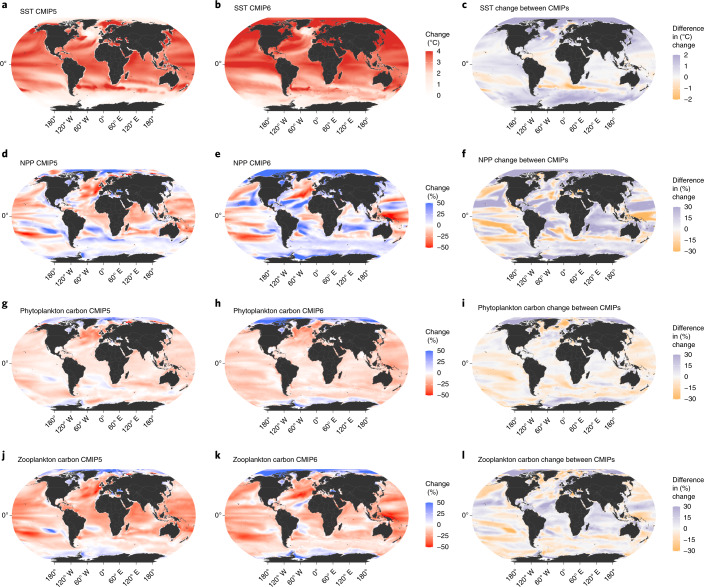
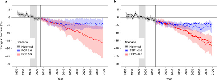
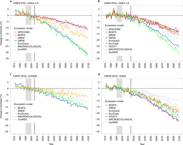
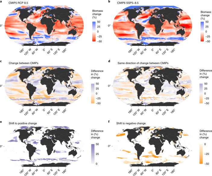
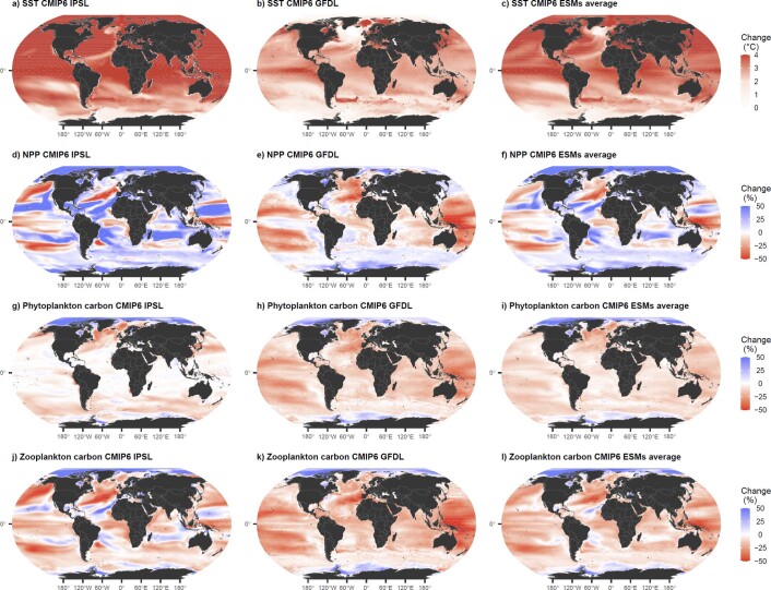
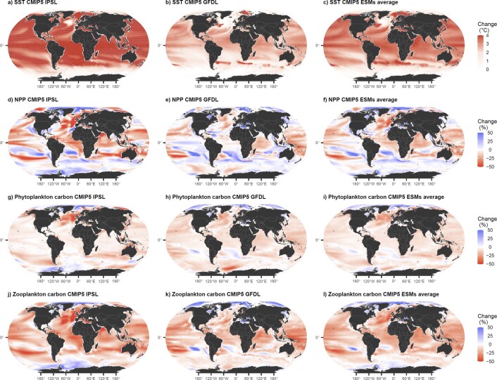
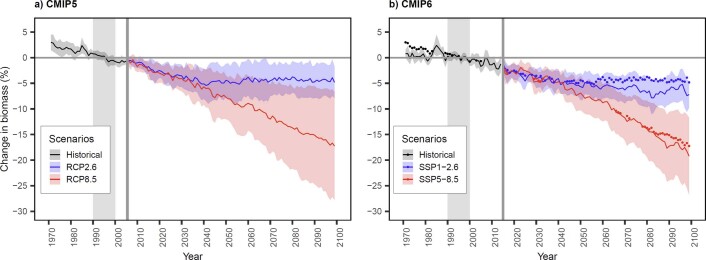
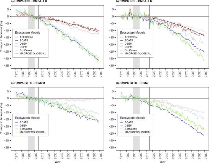
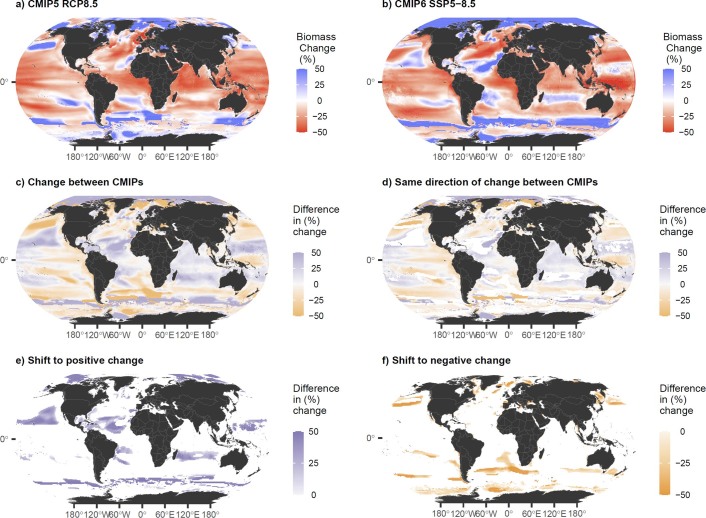
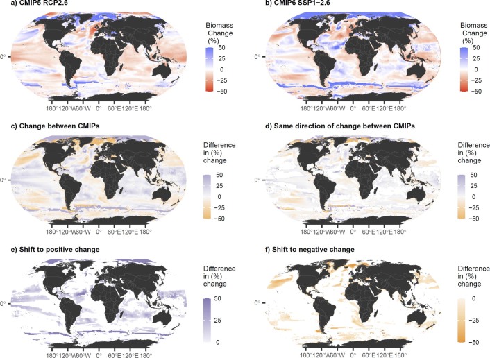
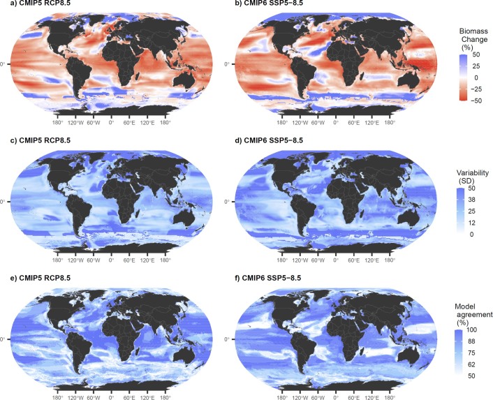
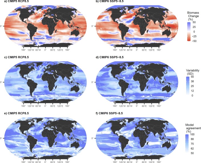
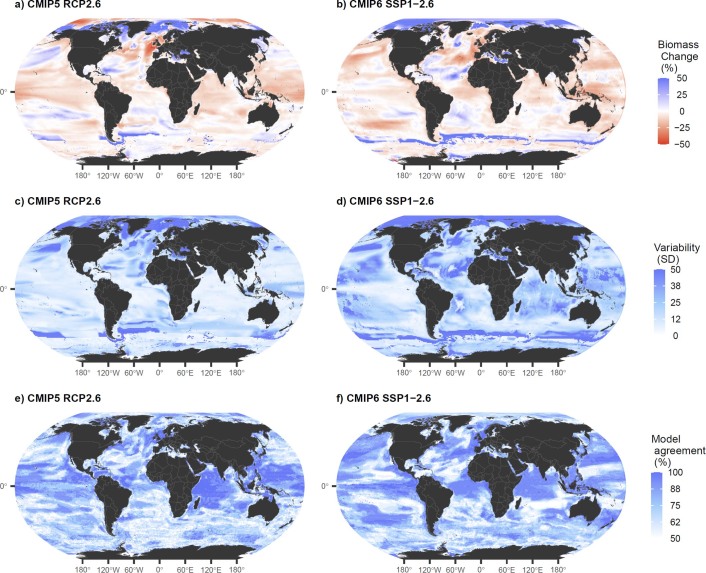
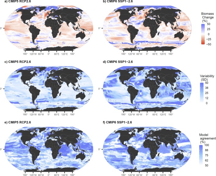
Projections of climate change impacts on marine ecosystems have revealed long-term declines in global marine animal biomass and unevenly distributed impacts on fisheries. Here we apply an enhanced suite of global marine ecosystem models from the Fisheries and Marine Ecosystem Model Intercomparison Project (Fish-MIP), forced by new-generation Earth system model outputs from Phase 6 of the Coupled Model Intercomparison Project (CMIP6), to provide insights into how projected climate change will affect future ocean ecosystems. Compared with the previous generation CMIP5-forced Fish-MIP ensemble, the new ensemble ecosystem simulations show a greater decline in mean global ocean animal biomass under both strong-mitigation and high-emissions scenarios due to elevated warming, despite greater uncertainty in net primary production in the high-emissions scenario. Regional shifts in the direction of biomass changes highlight the continued and urgent need to reduce uncertainty in the projected responses of marine ecosystems to climate change to help support adaptation planning.

Keywords: Climate-change ecology; Ecological modelling; Marine biology.

Fig. 1. Projected mean global change in oceanographic properties from IPSL and GFDL ESMs.

a–h, Rows depict SST (a,b), NPP (c,d), phytoplankton carbon (e,f) and zooplankton carbon (g,h) for GFDL and IPSL CMIP5 and CMIP6 under strong-mitigation (blue) and high-emissions (red) scenarios. Historical values (1970–2005 for CMIP5; 1970–2014 for CMIP6) are shown in black, and projections (2006–2099 for CMIP5; 2015–2099 for CMIP6) are coloured. All values are normalized relative to the period 1990–1999. Vertical grey shaded area indicates reference decade, and vertical grey line indicates first year of projection (subsequent to historical period). RCP, representative concentration pathway.

Fig. 2. Projected mean spatial changes in oceanographic properties.

a–l, Rows depict SST (a–c), NPP (d-f), phytoplankton carbon (g–i) and zooplankton carbon (j–l) for 1990–1999 and 2090–2099. Maps represent mean change for GFDL and IPSL models under a high-emissions scenario. Columns depict mean change under CMIP5 (a,d,g,j), mean change under CMIP6 (b,e,h,k) and the difference in these century changes between CMIP6 and CMIP5 (c,f,i,l), with a positive value indicating a stronger increase (or weaker decrease) in CMIP6, a negative value indicating a weaker increase (or stronger decrease) in CMIP6 and zero representing an equal change projected in both CMIP5 and CMIP6.

Fig. 3. Multimodel mean change in marine animal biomass under strong-mitigation and high-emissions scenarios.

a, CMIP5. b, CMIP6. Blue colouring represents strong mitigation, and red represents high emissions. Coloured dots indicate years with higher ensemble means for CMIP5. All values relative to standardized reference period (1990–1999). Solid coloured lines indicate ensemble means; shaded areas indicate inter-model standard deviation. Vertical grey shaded area and line indicate reference decade and first year of projection after historical period, respectively. The full ensemble of MEMs is included for CMIP5 (7 models using IPSL and 5 models using GFDL, n = 12) and CMIP6 (9 models using IPSL and 7 models using GFDL, n = 16).

Fig. 4. Projected global change in marine animal biomass from individual MEMs driven by IPSL and GFDL under the high-emissions scenario.

a, CMIP5 IPSL-CM5A-LR. b, CMIP6 IPSL-CM6A–LR. c, CMIP5 GFDL-ESM2M. d, CMIP6 GFDL-ESM4M. A different set of MEMs is included for CMIP5 (7 models using IPSL and 5 models using GFDL, n = 12) and CMIP6 (9 models using IPSL and 7 models using GFDL, n = 16). All values are relative to the standardized reference period of 1990–1999. Vertical grey shaded area indicates reference decade, and vertical grey line indicates first year of projection subsequent to historical period.

Fig. 5. Ensemble mean change in marine animal biomass under the high-emissions scenario.

The full ensemble of MEMs is included for CMIP5 (7 models using IPSL and 5 models using GFDL, n = 12) and CMIP6 (9 models using IPSL and 7 models using GFDL, n = 16). a,b, Maps represent mean percentage change between 1990–1999 and 2090–2999 under CMIP5 (a) and CMIP6 (b). c, Difference in percentage change between CMIP5 and CMIP6. d, Difference in percentage change between CMIP5 and CMIP6 for grid cells showing same direction of change. e, Difference in percentage change between CMIP5 and CMIP6 for grid cells changing from CMIP5 decrease to CMIP6 increase. f, Same as in e for grid cells changing from CMIP5 increase to CMIP6 decrease.

Extended Data Fig. 1. Spatial change in oceanographic properties under CMIP6 SSP5-8.5.

Change in sea -surface temperature (a-c), net primary production (d-f), phytoplankton carbon (g-i) and zooplankton carbon (j-l) between 1990–1999 and 2090–2099. Left column shows the mean change for IPSL-CM6A-LR. Middle column shows the mean change for GFDL-ESM4. Rightmost column shows the mean change averaged across GFDL and IPSL.

Extended Data Fig. 2. Spatial change in oceanographic properties under CMIP5 RCP8.5.

Change in sea surface temperature (a-c), net primary production (d-f), phytoplankton carbon (g-i) and zooplankton carbon (j-l) between 1990–1999 and 2090–2099. Left column shows the mean change for IPSL-CM5A-LR. Middle column shows the mean change for GFDL-ESM2M. Rightmost column shows the mean change averaged across GFDL and IPSL.

Extended Data Fig. 3. Multi-model change in marine animal biomass across comparable set of six marine ecosystem models (MEMs) run using both CMIP5 and CMIP6 forcings.

CMIP5 (a) and CMIP6 (b) results averaged across GFDL and IPSL under strong-mitigation (blue) and high-emissions (red) scenarios. Solid lines indicate ensemble model means; shaded areas indicate + /- inter-model standard deviation (n = 10; two MEMs only used IPSL). All values are relative to the standardized reference period of 1990–1999 (vertical grey shaded area). Vertical grey shaded area indicates reference decade and vertical grey line indicates first year of projection (subsequent to historical period). For the suite of MEMs considered, see Fig. 4. Coloured dots indicate CMIP5 values in years in which the ensemble mean values were higher for CMIP5 than for CMIP6.

Extended Data Fig. 4. Projected global change in marine animal biomass across comparable set of six marine ecosystem models (MEMs) run using both CMIP5 and CMIP6 forcings under the high-emissions scenario.

MEM outputs using CMIP5 (a & c) and CMIP6 (b & b) forcings (n = 10; two MEMs only used IPSL). All values are relative to the standardized reference period of 1990–1999. Vertical grey shaded area indicates reference decade and vertical grey line indicates first year of projection (subsequent to historical period).

Extended Data Fig. 5. Ensemble mean change in marine animal biomass across comparable set of six marine ecosystem models (MEMs) that used both CMIP5 and CMIP6 forcings under the high-emissions scenario.

MEM outputs using CMIP5 (a) and CMIP6 (b) forcings from GFDL and IPSL (n = 10; two MEMs only used IPSL). Maps represent mean percentage change between 1990–1999 and 2090–2999 under a) CMIP5 and b) CMIP6; c) difference in percentage change between CMIPs; d) difference in percentage change between CMIPs for grid cells that showed the same direction of change; e) difference in percentage change between CMIPs for grid cells that changed from a decrease in CMIP5 to an increase in CMIP6 and f) vice versa.

Extended Data Fig. 6. Ensemble mean change in marine animal biomass across comparable set of six marine ecosystem models (MEMs) that used both CMIP5 and CMIP6 forcings under the high-mitigation scenario.

MEM outputs using CMIP5 (a) and CMIP6 (b) forcings from GFDL and IPSL (n = 10; two MEMs only used IPSL). Maps represent mean percentage change between 1990–1999 and 2090–2999 under a) CMIP5 and b) CMIP6; c) difference in percentage change between CMIPs; d) difference in percentage change between CMIPs for grid cells that showed the same direction of change; e) difference in percentage change between CMIPs for grid cells that changed from a decrease in CMIP5 to an increase in CMIP6 and f) vice versa.

Extended Data Fig. 7. Ensemble model results from the full set of global marine ecosystem models under the high-emissions scenario.

Total consumer biomass change (a, b), inter-model standard deviation (c, d), and model agreement (e, f) where 100% represents all models indicating the same direction of change, and 50% indicates half the models indicating one direction of change and half indicating the opposite.

Extended Data Fig. 8. Ensemble model results from the comparable set of global marine ecosystem models that ran both CMIP5 and CMIP6 simulations under the high-emissions scenario.

Total consumer biomass change (a, b), inter-model standard deviation (c, d), and model agreement (e, f) where 100% represents all models indicating the same direction of change, and 50% indicates half the models indicating one direction of change and half indicating the opposite.

Extended Data Fig. 9. Ensemble model results from the full set of global marine ecosystem models under the strong-mitigation scenario.

Total consumer biomass change (a, b), inter-model standard deviation (c, d), and model agreement (e, f) where 100% represents all models indicating the same direction of change, and 50% indicates half the models indicating one direction of change and half indicating the opposite.

Extended Data Fig. 10. Ensemble model results from the comparable set of global marine ecosystem models that ran both CMIP5 and CMIP6 simulations under the strong-mitigation scenario.

Total consumer biomass change (a, b), inter-model standard deviation (c, d), and model agreement (e, f) where 100% represents all models indicating the same direction of change, and 50% indicates half the models indicating one direction of change and half indicating the opposite.

References

1. IPCC Special Report on the Ocean and Cryosphere in a Changing Climate (eds Pörtner, H.-O. et al.) (IPCC, 2019).
1. Doney SC, et al. Climate change impacts on marine ecosystems. Ann. Rev. Mar. Sci. 2012;4:11–37. doi: 10.1146/annurev-marine-041911-111611. - DOI - PubMed
1. Bindoff, N. L. et al. in Special Report on the Ocean and Cryosphere in a Changing Climate (eds Pörtner, H.-O. et al.) Ch. 5 (IPCC, 2019).
1. Griffith GP, Fulton EA, Gorton R, Richardson AJ. Predicting interactions among fishing, ocean warming, and ocean acidification in a marine system with whole-ecosystem models. Conserv. Biol. 2012;26:1145–1152. doi: 10.1111/j.1523-1739.2012.01937.x. - DOI - PubMed
1. Fu C, et al. Risky business: the combined effects of fishing and changes in primary productivity on fish communities. Ecol. Modell. 2018;368:265–276. doi: 10.1016/j.ecolmodel.2017.12.003. - DOI