. 2021 Nov 16;118(46):e2023832118.
doi: 10.1073/pnas.2023832118.

Drifting assemblies for persistent memory: Neuron transitions and unsupervised compensation

Affiliations

Drifting assemblies for persistent memory: Neuron transitions and unsupervised compensation

Yaroslav Felipe Kalle Kossio et al. Proc Natl Acad Sci U S A. .

Abstract

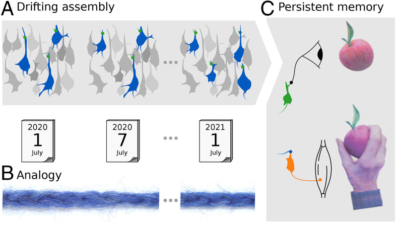
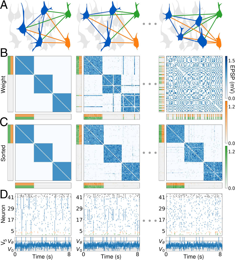
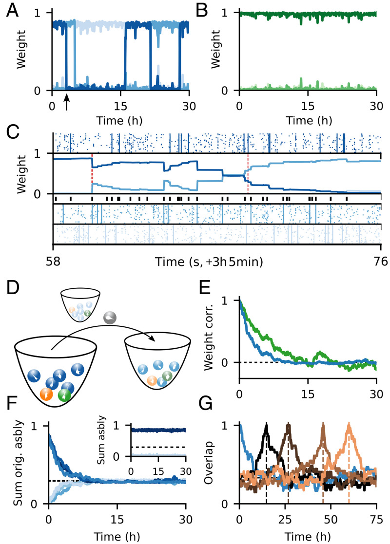
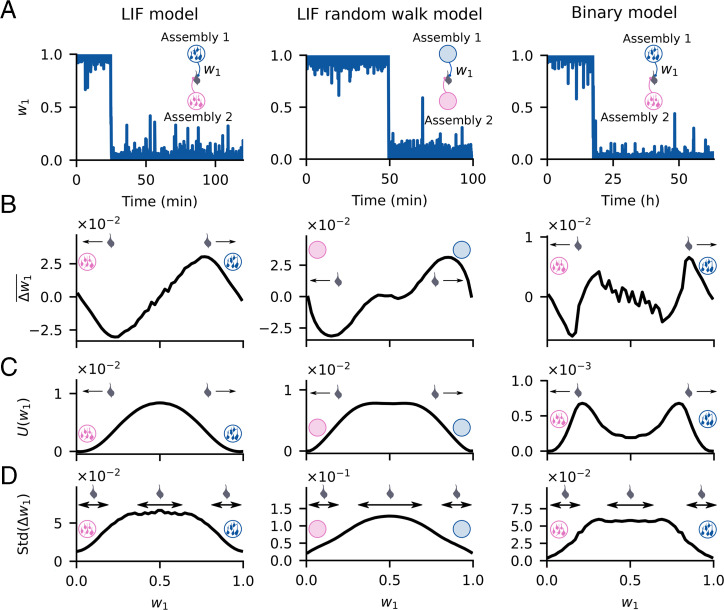
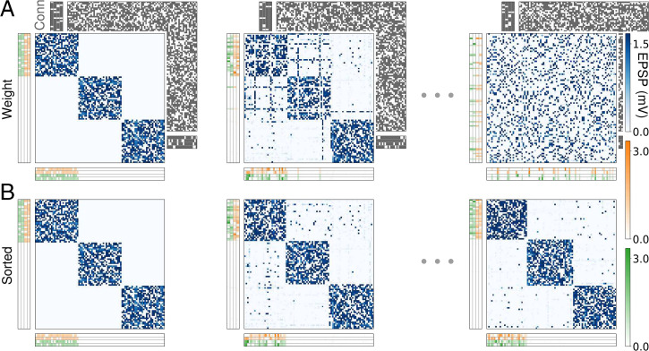
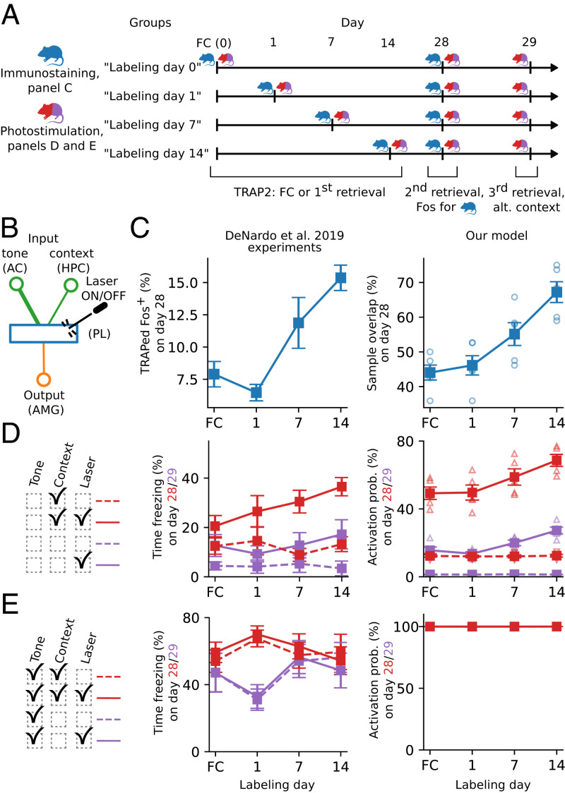
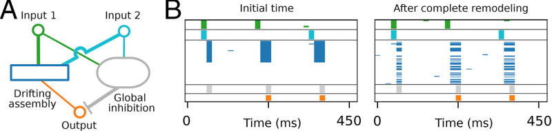
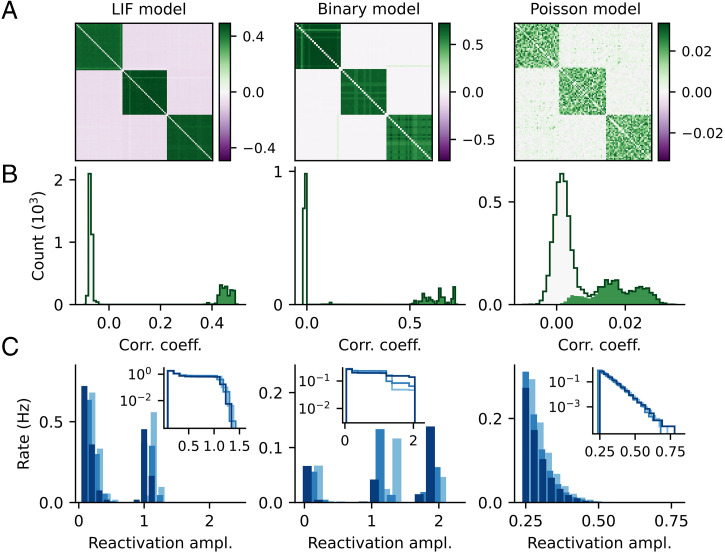
Change is ubiquitous in living beings. In particular, the connectome and neural representations can change. Nevertheless, behaviors and memories often persist over long times. In a standard model, associative memories are represented by assemblies of strongly interconnected neurons. For faithful storage these assemblies are assumed to consist of the same neurons over time. Here we propose a contrasting memory model with complete temporal remodeling of assemblies, based on experimentally observed changes of synapses and neural representations. The assemblies drift freely as noisy autonomous network activity and spontaneous synaptic turnover induce neuron exchange. The gradual exchange allows activity-dependent and homeostatic plasticity to conserve the representational structure and keep inputs, outputs, and assemblies consistent. This leads to persistent memory. Our findings explain recent experimental results on temporal evolution of fear memory representations and suggest that memory systems need to be understood in their completeness as individual parts may constantly change.

Keywords: associative memory; cell assemblies; neural representations; representational drift; synaptic remodeling.


Conflict of interest statement

The authors declare no competing interest.

Figures

Fig. 1
Fig. 1
Assembly drift and persistent memory. (A) At two nearby times a similar ensemble of neurons forms the neural representation of, for example, “apple” (compare the blue-colored assembly neurons at the first and the second time point). At distant times the representation consists of completely different ensembles (blue-colored assembly neurons at the first and the third time point). Due to their gradual change, temporally distant representations are indirectly related via ensembles in the time period between them. (B) Parts of a thread possess the same form of indirect relation: Nearby parts are composed of similar ensembles of fibers, while distant ones consist of different ensembles, which are connected by those in between. (C) The complete change of memory representations still allows for stable behavior. In the schematic, a tasty apple is perceived. At different times, this triggers different ensembles that presently form the representation of “apple”; see A. Assembly activation initiates a reaching movement toward the apple, despite the dissimilarity of the activated neuron ensembles. Memory and behavior are conserved because the gradual change of assembly neurons enables the inputs (green) and outputs (orange) to track the neural representation.
Fig. 2
Fig. 2
Drifting assemblies in spiking neural networks. (A) Schematics emphasizing strong synaptic coupling. While an assembly drifts freely (blue-colored assembly neurons) within the interior neurons, its input and output neurons (green and orange) follow it by adapting their synaptic weights. (B) Weights between interior neurons (blue weight matrix), from input and output neurons to the interior neurons (green and orange vertical weight matrices) and from the interior to the input and output neurons (green and orange horizontal weight matrices). Input (output) weights of neuron i are displayed as the ith row (column). Only weights of the four periphery neurons initially (and thus for all times) attached to assembly 1 are shown for clarity. Left column: Network initialization with three assemblies. Center column, after 27 min: Noisy autonomous spiking activity has already driven several interior neurons to attach to a new assembly (blue weight matrix, horizontal and vertical “lines” indicating the changed input and output preference). Right column, after 30 h: The assemblies have drifted away, and the weight matrix is completely remodeled. (C) Like B but with neurons reordered according to assemblies that they belong to, using a clustering algorithm. The assemblies remain intact and the periphery neurons stay strongly coupled to assembly 1. (D, Upper) Spike trains of the input (green) and output (orange) neurons of assembly 1, of 12 neurons from each of the ensembles that initially form assembly 1 (5 to 16), 2 (17 to 28) and 3 (29 to 40) and of 4 inhibitory neurons (black). (D, Lower) Membrane potential of the first interior neuron fluctuates irregularly. Spikes are marked by vertical lines above threshold Vθ; reset is to V0.
Fig. 3
Fig. 3
Analysis of drifting assemblies and their periphery neurons. (A) Switching of interior neurons in a simulation. Normalized summed weights between a neuron and current assemblies 1, 2, and 3 (dark to light blue) show temporary membership and fast transitions. (B) Periphery neurons stay attached to their assembly. Display is like A, with green colors indicating periphery neuron-assembly weights. (C) Closeup of the switching event indicated in A by an arrow. Raster plots: spikes of neurons in the three assemblies. The switching neuron is in assembly 1 (first subpanel) before and in assembly 2 after its transition. Second subpanel: total weight between each assembly and the neuron. Red dashed line, switching neuron spikes together with reactivation of assembly 2; light red dashed line, failure to spike with assembly 1. Third subpanel: Spikes of the switching neuron. (D) Schematic illustration of the mechanism underlying assembly drift. Noise drives balls (neurons) out of wells, which are generated by the different assemblies. They move to other wells (neurons switch assemblies). Periphery neurons (green, orange) experience too little noise to be pushed out of the wells; they stick with their assemblies. (E) Complete network weight remodeling. Pearson correlations between initial and later weights of interior (blue) and periphery-interior synapses (green) converge to chance level (black dashed line, 0). (F) Complete assembly remodeling. Summed weights within and between (darker and lighter blues) the three initial assemblies converge to chance level (1/3 of recurrent interior coupling, black). Inset shows maintenance of representational structure. Displayed is the sum of weights within current assembly 1 (dark blue) and between it and the current other two assemblies (light blue colors). (G) Assembly drift continues over time. Displayed is the overlap between the neuron ensemble forming assembly 1 at a reference time, with the neuron ensembles forming assembly 1 at other times. Reference times (dashed vertical lines) are initialization (blue curve) and first to fourth complete remodeling times (dark to light brown curves). Chance level is 1/3 (black, mostly covered).
Fig. 4
Fig. 4
Mechanisms of neuron transitions between assemblies driven by weight changes due to noisy autonomous activity. The mechanisms for the LIF model (A–D, Left) are well captured by a random walk model (A–D, Center); the mechanisms of the binary model (A–D, Right) are similar. (A) Long-term membership of a neuron in assemblies and fast transition between them. Large summed input weight w1 from assembly 1 to the neuron reflects membership in this assembly. (B) Average change Δw1¯ of the summed input weight w1 from assembly 1, as a function of the current weight value. (C) Corresponding potential U(w1) for the average weight changes. The average weight changes are roughly similar to the displacement of an object jumping down the landscape given by U(w1). (D) SD Std(Δw1) of the change of the summed input weight w1 from assembly 1, as a function of the current weight value. The two wells near 0 and 1 in (C and D) induce metastable states corresponding to the different assembly memberships.
Fig. 5
Fig. 5
Spontaneous synaptic turnover gives rise to assembly drift. (A) The matrix in the background shows the incomplete and spontaneously changing connectivity that drives the drift (gray: present synapses). Left column shows the weight and connectivity matrices after initialization, Center column shows those after 1 h, and Right column shows those after 37 h. Otherwise the depiction is like in Fig. 2B. (B) Like Fig. 2C.
Fig. 6
Fig. 6
Evolution of fear memory representation observed experimentally in ref. and drifting assembly model. (A) Schematics of the experiment. Immunostaining and photostimulation were conducted in different groups of mice. Immunostaining groups had two retrievals: first on day 1, 7, or 14 and second on day 28. Photostimulation groups had an additional retrieval on day 29 in an alternative context. (B) Model for the fear memory circuit with context input signaling conditioned cage from hippocampus (HPC), auditory stimulus input signaling conditioned tone from auditory cortex (AC), output to amygdala (AMG), and connecting drifting assembly in prelimbic cortex (PL). In some experiments a set of neurons in PL is photostimulated. Thicker line indicates stronger connection. (C, Left) Experimental data (8) that are proportional to the overlap of the memory representation directly after fear conditioning (FC, TRAPed neurons) or during first retrieval (on day 1, 7, or 14, TRAPed neurons), with the representation at the second retrieval (day 28, Fos+ neurons). Shown is the fraction of Fos+ neurons that were also TRAPed, in percent. The time interval between the labelings decreases from left to right. (C, Right) Overlap of the memory assembly in our model at the beginning of the trial (FC) or on day 1, 7, or 14 (circles; squares connected by solid lines, mean), with the assembly on day 28. (D) Fear expression tested on day 28 in the conditioning context (red, context input on) and on day 29 in an alternate context (purple, context input off). Laser activating a sample of the memory representation labeled (TRAPed) on different days (as in C) was either on (upward triangles; squares connected by solid lines, mean) or off (downward triangles; squares connected by dashed lines, mean). (Center) Experiment. (Right) Our model. (E) Same as D but in presence of conditioned auditory stimulus (tone input on). (Right). Red squares and solid lines overlay purple and dashed ones. Graphs show mean ± SEM and data points.
Fig. 7
Fig. 7
Drifting XOR gate. (A) Schematics of the network setup. Two groups of input neurons (green and cyan) are connected via a drifting assembly (blue) to output neurons (orange). An inhibitory population (gray) inhibits all neurons. Thicker lines indicate stronger connection. Only projections and neuron populations that are directly relevant for the XOR computation are shown for clarity. (B) Functionality of the drifting XOR gate at two distant times. Activity of input 1 (green), input 2 (cyan), hidden layer (blue), inhibitory (gray), and output (orange) neurons is displayed by horizontal lines in different bars (from top to bottom). The interior neurons are indexed such that initially (Left) the XOR assembly activity fills the upper part of the third bar. Later, due to complete remodeling of the assembly, its activity is distributed all over the bar (Right). Functionality is nevertheless conserved: The output neurons become active if exactly one of the input neuron groups is active.
Fig. 8
Fig. 8
Spike correlations and assembly reactivations in our network models. (Left) LIF network of Fig. 2. (Center) Binary network (SI Appendix, Fig. S6). (Right) Poisson network (SI Appendix, Fig. S13). All networks have frozen connectivity and weights, which are obtained by fixing plastic networks after the first complete remodeling. (A and B) Correlations between Poisson neurons (Right) are much smaller than those in the other two networks (Left and Center). (A) Matrices of measured spike count correlation coefficients with neurons sorted according to their assembly membership. Diagonal entries (equal to one) are blanked in white. (B) Histograms of correlation coefficients. Solid line gives the full histogram over all neuron pairs. Green shading indicates the contribution from intraassembly neuron pairs and light shading the remaining contribution from pairs of neurons belonging to different assemblies. (C) Assembly reactivation is absent in Poisson networks. Main panels show how often different maxima of the number of spikes in a moving time window are detected within an assembly (Materials and Methods). Occurrence rate is plotted against number of spikes divided by the assembly size (different blue colors for the assemblies). Events of spontaneous assembly reactivation are reflected by a second peak, separate from the background continuum near zero. Insets show the complementary cumulative distributions with logarithmic rate scale.

Similar articles

Cited by

References

    1. Rumpel S., Triesch J., The dynamic connectome. e-Neuroforum 22, 48–53 (2016).
    1. Humeau Y., Choquet D., The next generation of approaches to investigate the link between synaptic plasticity and learning. Nat. Neurosci. 22, 1536–1543 (2019). - PubMed
    1. Yasumatsu N., Matsuzaki M., Miyazaki T., Noguchi J., Kasai H., Principles of long-term dynamics of dendritic spines. J. Neurosci. 28, 13592–13608 (2008). - PMC - PubMed
    1. Rubinski A., Ziv N. E., Remodeling and tenacity of inhibitory synapses: Relationships with network activity and neighboring excitatory synapses. PLOS Comput. Biol. 11, e1004632 (2015). - PMC - PubMed
    1. Dvorkin R., Ziv N. E., Relative contributions of specific activity histories and spontaneous processes to size remodeling of glutamatergic synapses. PLoS Biol. 14, e1002572 (2016). - PMC - PubMed

Publication types