A cloud-based toolbox for the versatile environmental annotation of biodiversity data

Abstract

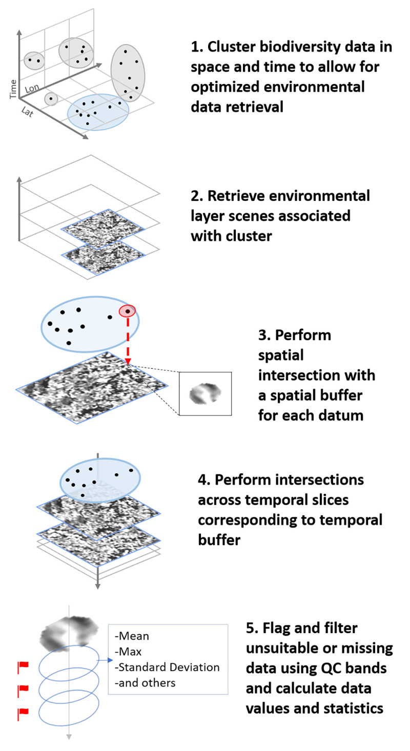
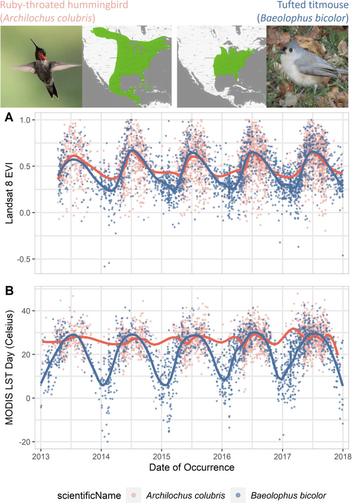
A vast range of research applications in biodiversity sciences requires integrating primary species, genetic, or ecosystem data with other environmental data. This integration requires a consideration of the spatial and temporal scale appropriate for the data and processes in question. But a versatile and scale flexible environmental annotation of biodiversity data remains constrained by technical hurdles. Existing tools have streamlined the intersection of occurrence records with gridded environmental data but have remained limited in their ability to address a range of spatial and temporal grains, especially for large datasets. We present the Spatiotemporal Observation Annotation Tool (STOAT), a cloud-based toolbox for flexible biodiversity-environment annotations. STOAT is optimized for large biodiversity datasets and allows user-specified spatial and temporal resolution and buffering in support of environmental characterizations that account for the uncertainty and scale of data and of relevant processes. The tool offers these services for a growing set of near global, remotely sensed, or modeled environmental data, including Landsat, MODIS, EarthEnv, and CHELSA. STOAT includes a user-friendly, web-based dashboard that provides tools for annotation task management and result visualization, linked to Map of Life, and a dedicated R package (rstoat) for programmatic access. We demonstrate STOAT functionality with several examples that illustrate phenological variation and spatial and temporal scale dependence of environmental characteristics of birds at a continental scale. We expect STOAT to facilitate broader exploration and assessment of the scale dependence of observations and processes in ecology.

Fig 1

Variation in spatiotemporal characteristics of (A, B) biodiversity data and (C, D) ecological processes underlying biodiversity data. The blue cylinders reflect the spatiotemporal grain of the data itself, with the red and green cylinders reflecting data uncertainty and driver extent, respectively.

Fig 2. STOAT environmental annotation dashboard.

Here, a test dataset is set up for annotation against the MODIS Day LST layers. A constant 1,000-m buffer is used, reflecting the native resolution of the environmental data, whereas temporal buffers are varied. LST, Land Surface Temperature; STOAT, Spatiotemporal Observation Annotation Tool.

Fig 3. STOAT architecture.

STOAT, Spatiotemporal Observation Annotation Tool.

Fig 4. STOAT environmental annotation workflow. Clustering procedure (Step 1) is carried out only for occurrence datasets of sufficient size.

QC, Quality Control; STOAT, Spatiotemporal Observation Annotation Tool.

Fig 5

(A) Landsat 8 EVI and (B) MODIS Day LST associated with occurrences of the ruby-throated hummingbird (Archilochus colubris, pink) and tufted titmouse (Baeolophus bicolor, blue) over a 5-year period. Note the differentiation between species in occupied environmental space. A loess curve was fitted to each species for visual illustration purposes. Range maps from Map of Life (https://mol.org). The data underlying this figure may be found at https://doi.org/10.5281/zenodo.5208219. EVI, Enhanced Vegetation Index; LST, Land Surface Temperature.

Fig 6. Spatial grain size dependence of the ruby-throated hummingbird EVI niche across different levels of habitat heterogeneity.

The y axis and right-side histogram show the absolute difference in Landsat 8 EVI values (ΔEVI) between annotations conducted at 120 m and 990 m spatial grain (buffer). They are plotted in relation to a measure of landscape level (1 km) habitat heterogeneity (x axis, top histogram). Black lines show quantile regression fits (10%, 50%, and 90%) and illustrate how grain differences are smaller in more homogenous landscapes. Darker colors indicate greater point density. The data underlying this figure may be found at https://doi.org/10.5281/zenodo.5208219. EVI, Enhanced Vegetation Index.

Fig 7. Temporal grain size dependence of the tufted titmouse temperature (LST) niche across seasons.

The y axis and right-side histogram show the absolute difference in MODIS LST Day when annotating with a 1-day and 30-day temporal buffer. They are plotted against day of the year (x axis, top histogram). A fitted loess curve illustrates the seasonal trends in the temporal buffer differences. Darker colors indicate greater point density. The data underlying this figure may be found at https://doi.org/10.5281/zenodo.5208219. LST, Land Surface Temperature.

Fig 8. Comparison of record grain-specific and grain-agnostic annotation for Anna’s hummingbird.

The y axes show the difference or absolute difference in Landsat 8 EVI (ΔEVI) between an annotation conducted at a record’s original spatial grain (and a 32-day temporal buffer) versus the same record annotated at 1 km against a monthly (A) or long-term (B) EVI layer. (A) |ΔEVI| plotted against record spatial grain. |ΔEVI| increases as the spatial grain of the record deviates from the standard 1-km annotation grain. (B) ΔEVI plotted against day of the year. ΔEVI fluctuates seasonally, reaching a peak in the summer and bottoming out in the winter. Fitted loess curves are added to illustrate both trends. Darker colors indicate greater point density. The data underlying this figure may be found at https://doi.org/10.5281/zenodo.5208219. EVI, Enhanced Vegetation Index.

References

1. Bonney R, Shirk JL, Phillips TB, Wiggins A, Ballard HL, Miller-Rushing AJ, et al.. Next steps for citizen science. Science. 2014;343(6178):1436–7. doi: 10.1126/science.1251554 - DOI - PubMed
1. Chandler M, See L, Copas K, Bonde AMZ, Lopez BC, Danielsen F, et al.. Contribution of citizen science towards international biodiversity monitoring. Biol Conserv. 2017;213:280–94. 10.1016/j.biocon.2016.09.004. WOS:000410011900006. - DOI
1. Kays R, Crofoot MC, Jetz W, Wikelski M. Terrestrial animal tracking as an eye on life and planet. Science. 2015;348 (6240):aaa2478. doi: 10.1126/science.aaa2478 - DOI - PubMed
1. Mccallum J. Changing use of camera traps in mammalian field research: habitats, taxa and study types. Mammal Rev. 2013;43(3):196–206. 10.1111/j.1365-2907.2012.00216.x. WOS:000319982700004. - DOI
1. He KS, Bradley BA, Cord AF, Rocchini D, Tuanmu MN, Schmidtlein S, et al.. Will remote sensing shape the next generation of species distribution models? Remote Sens Ecol Con. 2015;1(1):4–18. 10.1002/rse2.7. WOS:000448239100002. - DOI
Publication types