Seasonal mixed layer depth shapes phytoplankton physiology, viral production, and accumulation in the North Atlantic

Abstract

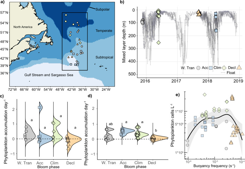
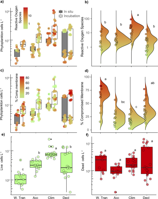
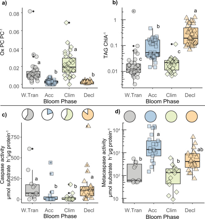
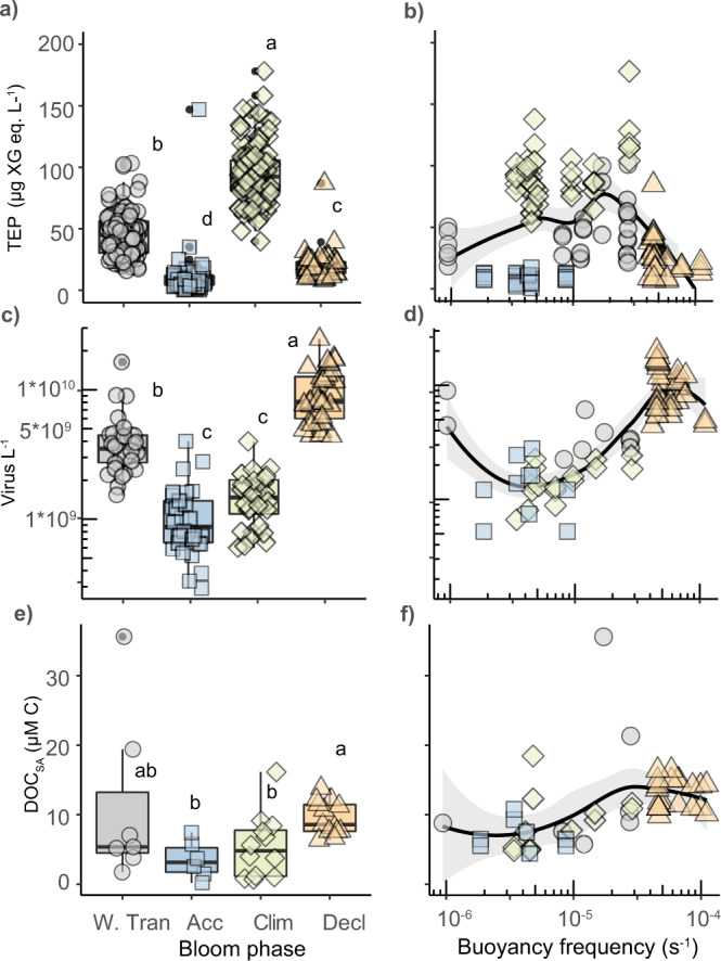
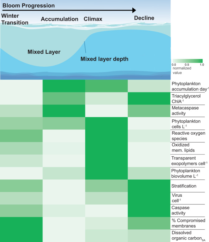
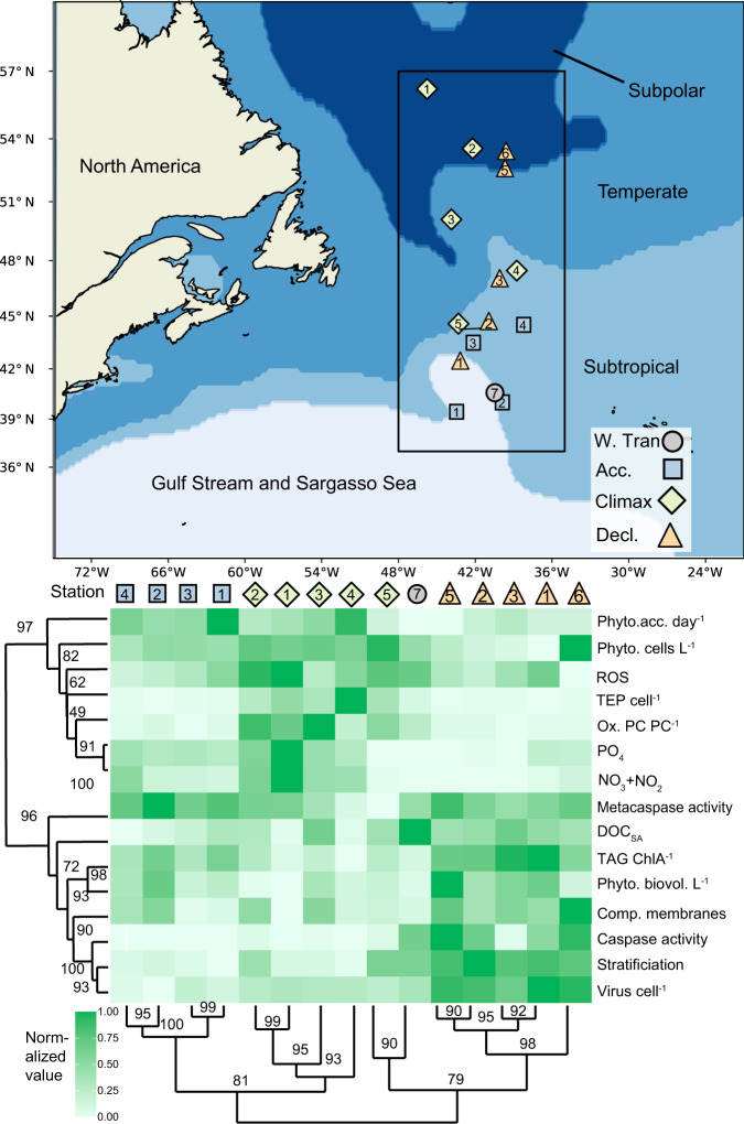
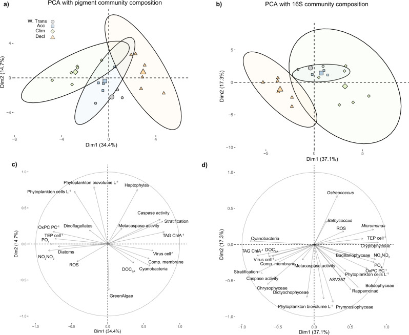
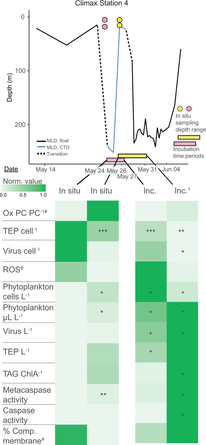
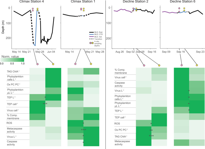
Seasonal shifts in phytoplankton accumulation and loss largely follow changes in mixed layer depth, but the impact of mixed layer depth on cell physiology remains unexplored. Here, we investigate the physiological state of phytoplankton populations associated with distinct bloom phases and mixing regimes in the North Atlantic. Stratification and deep mixing alter community physiology and viral production, effectively shaping accumulation rates. Communities in relatively deep, early-spring mixed layers are characterized by low levels of stress and high accumulation rates, while those in the recently shallowed mixed layers in late-spring have high levels of oxidative stress. Prolonged stratification into early autumn manifests in negative accumulation rates, along with pronounced signatures of compromised membranes, death-related protease activity, virus production, nutrient drawdown, and lipid markers indicative of nutrient stress. Positive accumulation renews during mixed layer deepening with transition into winter, concomitant with enhanced nutrient supply and lessened viral pressure.

Fig. 1. Mixed layer depth and phytoplankton accumulation dynamics.

a Locations of sampled stations within subregions of the Northwest Atlantic during the NAAMES expeditions (color coded and shaped by the bloom phase; W. Tran = Winter Transition; Acc = Accumulation; Clim = Climax; Decl = Decline; See key in Panel B). Black rectangle represents the study area of NAAMES and this research. b Mixed layer depths within the NAAMES campaigns (black box in Fig. 1a), calculated from CTD casts at each of the station locations (colored symbols) and Bio-ARGO profiling floats that were deployed at stations and sampled continuously (small circles with separate grey lines for each float). The latter provided a history of mixed layer depths before, during, and after occupation. c Bloom phase distribution of accumulation rates for in situ phytoplankton populations sampled several times per day at 5 m. Each point represents the median accumulation rate of each station. d Bloom phase distribution of phytoplankton cell accumulation rates derived from on-deck incubations of phytoplankton populations at simulated in situ light and temperature conditions (see ‘Methods’). Each point represents a biological replicate. Data in panels (c) and (d) are based on cell concentrations and contoured with ridgeline smoothing to represent the distribution of accumulation rates across stations within a given bloom phase. The size of contour peaks is driven by frequency of observations. e Phytoplankton concentration (taken from 5 m) as a function of water column stratification (expressed as buoyancy frequency; s⁻¹). Higher buoyancy frequencies to the right of the plot represent more stratification. A LOESS line of best fit (shaded area = 95% confidence interval) for data shows the general trend of phytoplankton concentration across all seasonal phases. Different letters denote statistically significant groups (p < 0.05, Kruskal−Wallis test with Dunn corrections for multiple comparisons). Intergroup comparisons with more than one letter denote no significant difference between the two groups. Similar analyses as those presented in panels (c)−(e) are presented for phytoplankton biovolume in Supplementary Fig. 1. Exact p values and number of biological replicates can be found in Source Data file.

Fig. 2. Seasonal phases have distinct physiological state signatures.

a, c Concentration of phytoplankton cells sampled within the mixed layer at depths associated with 40, 20, or 1% surface irradiance during different seasonal phases (W.Tran = Winter Transition; Acc = Accumulation; Clim = Climax; Decl = Decline). Data are shown for in situ water (grey bars) and on-deck incubations (open bars). Population-wide levels of a, b cellular reactive oxygen species (colored by fluorescence fold change from unstained; median per population) and c, d cell death (colored by % compromised membrane). Plots (b) and (d) are contoured with ridgeline smoothing to represent the relative in situ distribution of biomarker levels within each phase. The size of contour peaks is driven by frequency of observations. e, f In situ inventories of live (e; green) and dead (f; red) cells within the mixed layer through the different phases. Individual circles denote biological replicates. Box plots in (a), (c), (e) and (f) represent the median value bounded by the upper and lower quartiles with whiskers representing median + quartile × 1.5. Different letters denote statistically significant groups (p < 0.05, Kruskal−Wallis test with Dunn corrections for multiple comparisons). Intergroup comparisons with more than one letter denote no significant difference between the two groups. Number of biological replicates, by bloom phase/cast type (from left to right) = 10/9, 13/33, 17/36, 19/36 (a), 11/25, 13/36, 17/36, 19/36 (c), 11, 13, 17, 19 (e, f). Exact p values can be found in Source Data file.

Fig. 3. Seasonal phases are characterized by distinct lipid profiles and cell death-associated proteolytic activity.

a Oxidized phosphatidylcholine (OxPC40:10, OxPC42:11, OxPC44:12) normalized to total phosphatidylcholine (PC40:10, PC42:11, PC44:12). b Triacylglycerol (TAG; pmol L⁻¹), normalized to ChlA (peak area/L). c (top) The proportion of in situ samples with positive caspase activity (cleavage of IETD-AFC; color shading). (bottom) Caspase-specific activity rates (µmol substrate hydrolyzed h⁻¹ µg protein⁻¹) for in situ populations. d (top) The proportion of in situ samples with positive metacaspase activity (cleavage of VRPR-AMC; color shading). (bottom) Metacaspase-specific activity rates (µmol substrate hydrolyzed h⁻¹ µg protein⁻¹) for in situ populations. All box plots represent the median value bounded by the upper and lower quartiles, with whiskers representing median + quartile × 1.5. Different letters denote statistically significant groups (p < 0.05, Kruskal−Wallis test with Dunn corrections for multiple comparisons). Intergroup comparisons with more than one letter denote no significant difference between the two groups. Lipids and enzyme activities derived from biomass collected within the mixed layer at depths associated with 40, 20, or 1% surface irradiance (see ‘Methods’). Individual symbols in all panels represent biological replicates and are colored and shaped by bloom phase. Seasonal phases are indicated in each panel (W.Tran = Winter Transition; Acc = Accumulation; Clim = Climax; Decl = Decline). Number of biological replicates, by bloom phase (from left to right) = 35, 37, 31, 36 (a), 35, 41, 36, 35 (b), 11, 15, 15, 20 (c), 11, 17, 14, 20 (d). Exact p values can be found in Source Data file.

Fig. 4. Seasonal phases are characterized by distinct extracellular signatures in aggregation potential, virus particle concentration, and DOC accumulation.

Concentrations of a, b transparent exopolymer particles (TEP: µg Xanthan Gum equivalents L⁻¹), c, d virus-like particles (Virus L⁻¹), and e, f seasonally accumulated dissolved organic carbon (DOC_SA: μM carbon) within the mixed layer at depths corresponding to 40, 20, or 1% surface irradiance for different seasonal phases (W.Tran = Winter Transition; Acc = Accumulation; Clim = Climax; Decl = Decline). Panels (b), (d), (f) show a subset of samples (corresponding to 5 m sampling depth) plotted as a function of water column stratification (LOESS, shaded area = 95% confidence interval) (buoyancy frequency; s⁻¹). Lower buoyancy frequency values to the right of the plot are more stratified. Individual symbols represent biological replicates and are shaped and colored by bloom phase. Box plots represent the median value bounded by the upper and lower quartiles with whiskers representing the median + quartile × 1.5 Different letters denote statistically significant groups (p < 0.05, Kruskal−Wallis test with Dunn corrections for multiple comparisons). Intergroup comparisons with more than one letter denote no significant difference between the two groups. Number of biological replicates, by bloom phase (from left to right) = 95, 73, 101, 55 (a), 30, 32, 32, 32 (c), 7, 6, 12, 12 (e). Exact p values can be found in Source Data file.

Fig. 5. Biomarkers of physiological state cluster according to bloom phase and stratification.

(Top) Conceptual illustration of changes in mixed layer depths and water column stratification associated with seasonal bloom phases in the North Atlantic. (Bottom) Heatmap of different biomarkers (organized as rows). Row shading represents the median of each variable throughout a phase, normalized to the entire cycle. Rows are clustered by an optimal leaf algorithm to minimize the distance between normalized distributions of each variable (leaves). Phytoplankton accumulation day⁻¹ = cell concentration-based accumulation rate (day⁻¹); Triacylglycerol ChlA⁻¹ = triacylglycerol concentration (pM) normalized to chlorophyll A; Metacaspase activity = µmol metacaspase substrate cleaved h⁻¹ µg protein⁻¹; Phytoplankton cells L⁻¹ = phytoplankton concentration (cells L⁻¹); Reactive oxygen species = log₁₀ fold change from unstained phytoplankton population; Oxidized mem. lipids = oxidized phosphatidylcholine normalized to total phosphatidylcholine; Transparent exopolymers cell⁻¹ = transparent exopolymer particles (µg XG eq. L⁻¹) normalized to bacteria and phytoplankton cell concentrations; Phytoplankton biovolume L⁻¹ = phytoplankton biovolume (µL L⁻¹); Stratification = measured buoyancy frequency (s⁻¹); Virus cell⁻¹ = virus concentration normalized to phytoplankton and bacterial cell concentrations; Caspase activity = µmol caspase substrate cleaved h⁻¹ µg protein⁻¹; % Compromised membranes = % of phytoplankton population with compromised membranes; Dissolved organic carbon_SA = seasonally accumulated dissolved organic carbon (µM change from minimum value per bloom phase).

Fig. 6. Comparison of biomarker signatures between stations and bloom phases in the NAAMES study area.

(Top) Map of stations within subregions and bloom phases used in this analysis. Only stations with in situ values of all of the biomarkers in the heatmap below were included, except for accumulation rates, which were calculated from on-deck incubations. Stations with more than one sampling date were consolidated into a single latitude and longitude for the purpose of this map. Stations are shaped and colored by bloom phase:W. Tran = Winter Transition, Acc. = Accumulation, Climax, Decl. = Decline. (Bottom) Heatmap of normalized values of biomarkers throughout the bloom. The median value at each station, within the mixed layer was normalized to the highest and lowest median values throughout the bloom. Dendrogram clustering was done with the average method, using a correlation distance matrix of normalized values. Bootstrap values (n = 1000) are pvclust’s AU p value—higher is more significant. Rows and columns were ordered using Dendrogram cluster order. Phytoplankton acc. day⁻¹ = cell concentration-based accumulation rate (day⁻¹); Phyto. cells L⁻¹ = phytoplankton concentration (cells L⁻¹); ROS = Reactive oxygen species (log₁₀ fold change from unstained); TEP cell⁻¹ = transparent exopolymer particle concentration (µg XG eq. L⁻¹) normalized to phytoplankton and bacteria concentrations; Ox.PC PC⁻¹ = oxidized phosphatidylcholine normalized to total phosphatidylcholine; PO₄ = phosphate concentration (µM); NO₃ + NO₂ = nitrate plus nitrite concentration (µM); Metacaspase activity = µmol metacaspase substrate cleaved h⁻¹ µg protein⁻¹; DOC_SA = seasonally accumulated dissolved organic carbon (µM change from minimum value per bloom phase); TAG ChlA⁻¹ = triacylglycerol (µM) normalized to Chlorophyll A peak area/L; Phyto. biovol. L⁻¹ = phytoplankton biovolume (µL L⁻¹); Comp. membranes = % of population with compromised membranes; Caspase activity = µmol caspase substrate cleaved h⁻¹ µg protein⁻¹; Stratification = measured water column buoyancy frequency (s⁻¹); Virus cell⁻¹ = virus concentrations normalized to phytoplankton and bacteria concentrations.

Fig. 7. Principle component analysis associates bloom phases with distinct physiological states and extracellular signatures.

(Top row) PCA showing interrelationships among measured intra- and extracellular properties for phytoplankton populations across bloom seasons combined with clade relative abundance determined by either a Pigment-based community composition or b 16S rRNA-based community composition. Symbols are shaped and colored by station. Small symbols represent individual sampling events during each bloom phase; large symbols represent the average value for each respective bloom phase. Percent variability in each dimension is the amount of variance explained in the dataset. Ellipses represent the 95% concentration estimate. W.Tran = Winter Transition; Acc = Accumulation; Clim = Climax; Decl = Decline. (Bottom row) PCA scores and vectors for measured intra- and extracellular properties with respect to c Pigment-based community composition and d 16S rRNA-based community composition. Longer arrows represent a stronger correlation with each respective dimension. Phytoplankton cells L⁻¹ = phytoplankton cell concentration; ROS = reactive oxygen species in phytoplankton (log₁₀ fold change in fluorescence from unstained); Comp. membrane = % of phytoplankton population with compromised membranes; TEP cell⁻¹ = transparent exopolymer particle concentration (µg XG eq. L⁻¹) normalized to bacteria and phytoplankton concentration; Virus cell⁻¹ = virus concentration normalized to bacteria and phytoplankton concentrations; OxPC PC⁻¹ = oxidized phosphatidylcholine (peak area) normalized to total phosphatidylcholine; TAG ChlA⁻¹ = triacylglycerol (pM) normalized to ChlA (peak area/L); Caspase activity = caspase activity (µmol caspase substrate cleaved h⁻¹ µg protein⁻¹); Metacaspase activity = metacaspase activity (µmol metacaspase substrate cleaved h⁻¹ µg protein⁻¹); DOC_SA = seasonally accumulated dissolved organic carbon; Phytoplankton biovolume L⁻¹ = phytoplankton µl L⁻¹; Stratification = stratification of the upper 300 m, expressed as buoyancy frequency (s⁻¹). Biomarkers are plotted according to their co-variability with phytoplankton groups defined by pigments (i.e., Green Algae, Cyanobacteria, Diatoms, Dinoflagellates, Haptophytes) or 16S (i.e., Cyanobacteria, Chrysophyceae, Dictyochophyceae, Prymnesiophyceae, Rappemonad, Bolidophyceae, ASV357, Bacillariophyceae, Cryptophyceaea, Micromonas, Bathycoccus, Ostreococcus).

Fig. 8. Physiological state of phytoplankton transitioning from a deep to a shallow mixed layer.

(Top) Mixed layer depth at Climax Station 4 in relation to sampled phytoplankton communities. Solid black line represents mixed layer depth (MLD) pre- and post-occupation provided by drifting BioArgo floats (solid black line). A dashed line represents the transition from the float-measured MLD to ship-measured MLD (solid blue line), since sampling was done near and not directly at the float. Water sampled from the first and third days of occupation are indicated by pink and yellow symbols, respectively. The y axis positions of colored circles represent sampling depths. The x axis position of colored circles represents the date of sampling. Colored bars on the x axis correspond to incubation times of sampled communities (colored circles were the source water). (Bottom) Comparison of intra- and extracellular biomarkers from phytoplankton associated with in situ and incubation samples from above. Color shading in each row represents the normalized distribution of each parameter over the 8-day transition from a deeply mixed to a shallow mixed layer. Row order is clustered by optimal leaf algorithm. Data for incubations derive from the same in situ water collected on days 1 and 3, respectively, and incubated on deck at in situ light and temperature (see ‘Methods’). Asterisks indicate significant differences from day 1 via Kruskal−Wallis test (*p < 0.05, **p < 0.01, ***p < 0.001). Ox PC PC^{− 1} = oxidized phosphatidylcholine normalized to total PC; TEP cell⁻¹ = transparent exopolymer particles normalized to phytoplankton and bacterial cell concentrations; Virus cell⁻¹ = virus concentration normalized to phytoplankton and bacterial cell concentrations; ROS = reactive oxygen species; Phytoplankton cells L⁻¹ = phytoplankton cell concentration; Phytoplankton µl L⁻¹ = phytoplankton biovolume; Virus L⁻¹ = virus concentration; TEP L⁻¹ = transparent exopolymer concentration; TAG ChlA⁻¹ = triacylglycerol concentration (pM) normalized to chlorophyll A peak area/L; Metacaspase activity = µmol metacaspase substrate cleaved, µg protein⁻¹ h⁻¹; Caspase activity = µmol caspase substrate cleaved, µg protein⁻¹ h⁻¹; % Comp. membrane = % of population with compromised membranes. ¹Incubation samples from depths lower than 5 m were lost due to a storm knocking the incubation tanks off the deck. ^#n < 3 samples for at least 1 day for these parameters, due to loss of samples in transit or lack of sampling on day 1. See Supplementary Fig. 12 for raw parameter data from this station. Exact p values can be found in Source Data file.

Fig. 9. Inter-station comparisons of phytoplankton physiological state in water columns with different mixing depths and biomass loads.

(Top) Mixed layer depth dynamics at a subset of Climax and Decline stations in relation to sampled phytoplankton communities. Climax Station 4 transitioned from a deeply mixed to a shallow water column, while Climax Station 1 had more consistent MLDs during station occupation. More stable and shallow MLDs were observed during Decline phase, but phytoplankton communities had different relative biomass levels (Decline Station 6, high; Decline Station 2, low). Pre- and post-occupation mixed layer depths (MLD) are provided by drifting BioArgo floats (solid black line) or derived from satellite measurements (purple line), since BioArgo floats were not available for the Decline phase. A dashed line represents the transition from the float-measured MLD to ship-measured MLD (solid blue line), since sampling was done near and not directly at the float. y axis positions of colored circles represent sampling depths of in situ populations. x axis position of colored circles represents the date of sampling. Dates and data corresponding to colored symbols are used in the comparison table below. (Bottom) Comparison of intra- and extracellular biomarkers for phytoplankton associated with in situ samples from above. Pink symbols =  first day of occupation. Yellow symbols = subsequent day of occupation. Rows represent a two-day time course of each measured biomarker variable. Color shading represents the normalized distribution of each parameter within each seasonal phase to better illustrate relative responses to MLD dynamics. Row order is clustered by optimal leaf algorithm. Asterisks indicate significant differences between stations, via Kruskal−Wallis test (*p < 0.05, **p < 0.01, ***p < 0.001). Biomarker definitions are the same as in Fig. 8. OxPC PC⁻¹ also used additional data from the 1% light depth due to some samples being lost in transit. See Supplementary Fig. 13 for raw parameter data from these stations. Exact p values be found in Source Data file.

References

1. Bar-On YM, Phillips R, Milo R. The biomass distribution on Earth. Proc. Natl Acad. Sci. USA. 2018;115:6506–6511. - PMC - PubMed
1. Field CB, Behrenfeld MJ, Randerson JT, Falkowski P. Primary production of the biosphere: integrating terrestrial and oceanic components. Science. 1998;281:237–240. - PubMed
1. Valiela, I. Marine Ecological Processes (Springer, 1995).
1. Behrenfeld MJ, Boss ES. Student’s tutorial on bloom hypotheses in the context of phytoplankton annual cycles. Glob. Chang. Biol. 2018;24:55–77. - PMC - PubMed
1. Sverdrup HU. On conditions for the vernal blooming of phytoplankton. ICES J. Mar. Sci. 1953 doi: 10.1093/icesjms/18.3.287. - DOI
Publication types