Population receptive fields of human primary visual cortex organised as DC-balanced bandpass filters

Abstract

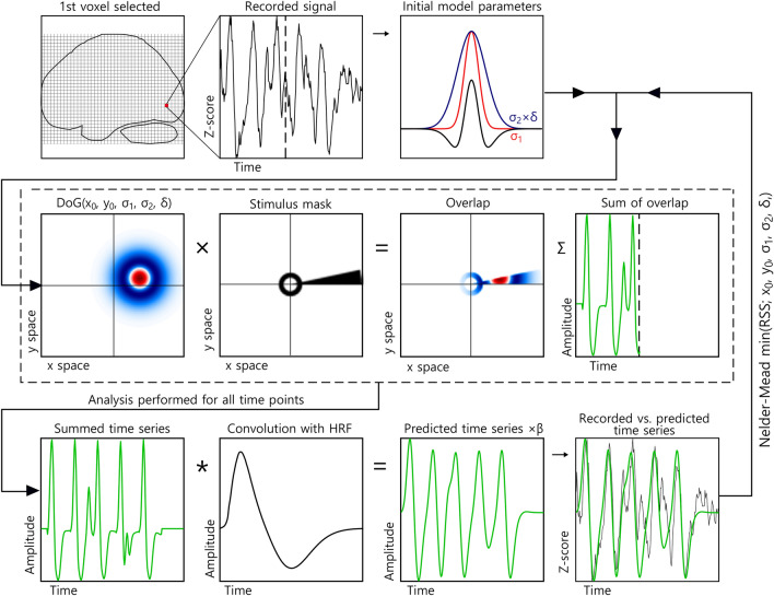
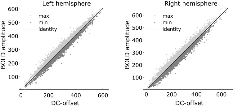
The response to visual stimulation of population receptive fields (pRF) in the human visual cortex has been modelled with a Difference of Gaussians model, yet many aspects of their organisation remain poorly understood. Here, we examined the mathematical basis and signal-processing properties of this model and argue that the DC-balanced Difference of Gaussians (DoG) holds a number of advantages over a DC-biased DoG. Through functional magnetic resonance imaging (fMRI) pRF mapping, we compared performance of DC-balanced and DC-biased models in human primary visual cortex and found that when model complexity is taken into account, the DC-balanced model is preferred. Finally, we present evidence indicating that the BOLD signal DC offset contains information related to the processing of visual stimuli. Taken together, the results indicate that V1 pRFs are at least frequently organised in the exact constellation that allows them to function as bandpass filters, which makes the separation of stimulus contrast and luminance possible. We further speculate that if the DoG models stimulus contrast, the DC offset may reflect stimulus luminance. These findings suggest that it may be possible to separate contrast and luminance processing in fMRI experiments and this could lead to new insights on the haemodynamic response.

Figure 1

Effects of filtering sinusoidal signals with Difference of Gaussians. (A) Sinusoidal signal with a frequency of 0.1 c/d The straight light grey line indicate DC offset. Inset, left: DC-balanced (black) and DC-biased (dark grey) DoG models in the spatial domain. Inset, right: Same as in the left inset, but in the frequency domain. The dashed vertical line indicates the frequency of the sinusoidal signal. (B) Sinusoidal signal after convolution with the two models in the insets. The dotted arrow from right inset to the signals in (B) shows the relation between the filter profile and the resulting signal.

Figure 2

pRF mapping procedure. The time series of one voxel is selected and initial model parameters are obtained from a simple coarse fitting procedure. The overlap between these parameters is then multiplied with a binary mask of the stimulus sequence, then summed for each TR. Convolution of the result and a haemodynamic response function is performed and scaled with β. This yields the final prediction for that particular combination of DoG model parameters, and this prediction is then compared with the recorded time series. Nelder-Mead minimization of RSS is then performed to find the best fitting DoG model parameters for each voxel.

Figure 3

Comparison of R² and AIC for the two models. (A) Mean R² for all participants’ left hemisphere (LH) and right hemisphere (RH) for the model without DC balance restriction (~ DC) and with DC balance restriction (DC) when all voxels had had R² > 0.05. The error bars indicate 95% confidence interval of the mean. (B) Percentage of voxels in the two hemispheres that exhibited a lower AIC score for the DC-balanced DoG model.

Figure 4

Comparison of fitted model parameters with computed model parameters according to Eq. (6). (A,B) Computed σ₁ plotted against original σ₁ for the left and right hemispheres. Light grey line shows the identity line. (C–F) Same as (A,B), but for σ₂ and δ.

Figure 5

Degree of bias for the unrestricted model. (A) All voxels sorted by the result given by Eq. (7). (B) Raincloud plot of the same bias-values as in A from − 5 to 5. The plot has been truncated to get a better view of the distribution. 92.16% of all voxels display − 5 > bias < 5. 75.62% of all voxels display − 1 > bias < 1. (C) Example of a DoG (blue) with a bias of -1.34 compared to a balanced model (black). (D) Same as (C), but with a bias of 4.14.

Figure 6

Comparison of R² and AIC for the two models using non-normalised data. (A) Mean R² for all participants’ left hemisphere (LH) and right hemisphere (RH) for the unrestricted model (~ DC) and with DC balance restriction (DC) when all voxels had had R² > 0.05 after being fitted to the non-normalised data. The error bars indicate 95% confidence interval of the mean. (B) Percentage of voxels in the two hemispheres that exhibited a lower AIC score for the DC-balanced DoG model using the non-normalised data.

Figure 7

DC-offset as a function of eccentricity. (A,B) Back-projection of the non-normalised DC offset data for a single participants’ left and right hemisphere, respectively. (C,D) Linear model (light grey) for DC offset as a function of eccentricity (log scale) for left and right hemisphere, respectively. The dark grey line indicates the moving average with a window size of 100 voxels.

Figure 8

Maximum and minimum BOLD response as a function DC offset. In both plots, the maximum BOLD amplitude is plotted as a function of DC offset is plotted in light grey, whereas the minimum BOLD response as a function of DC offset is plotted in dark grey. The identity line is shown in black.